Our goal in these next few chapters will be to develop a new definition of probability that is applicable in a broader range of settings than Bernoulli’s naive definition (Definition 1.4). In this brief chapter, we introduce some concepts from set theory that lay the foundation for what’s to come.
Set Operations
In the same way that operations on real numbers (e.g., addition, subtraction, inversion) take real numbers and return a new real number, set operations take events and return a new event. We introduce some standard set operations in this section. We will use the random babies experiment, which we recall below, as an illustrative example throughout.
Example A.1 (Returning random babies) Recall the generalized random babies experiment (Example 2.4) from Chapter 2, where we randomly return \(n\) babies to \(n\) sets of parents. We will suppose that the \(i\)th couple are biological parents of the \(i\)th baby and let \(E_i\) be the event that the \(i\)th couple gets their baby back. Labelling the couple that receives the \(i\)th baby as \(\omega_i\), we denote the experiment’s outcomes as \(\omega = (\omega_1, \dots, \omega_n)\). As an illustrative example, when \(n=3\), the outcome \((2, 1, 3)\) corresponds to the third couple getting their baby back and the first two couples swapping babies. This outcome is therefore in \(E_3\), but not in \(E_1\) or \(E_2\).
Intersection
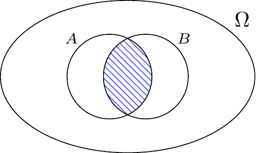
We start by defining the intersection of two events \(A\) and \(B\), which is itself the event that both \(A\) and \(B\) happen.
Definition A.1 (Intersection of two events) The intersection of events \(A\) and \(B\), denoted by \(A \cap B\), is the event that consists of any outcomes that are both in \(A\) and \(B\). Colloquially, we refer to the event \(A \cap B\) as \(A \and B\).
Example A.2 (First two babies returned correctly) The event \(E_1 \cap E_2\) is the event that both the first and second babies are returned to their biological parents. It is made up of all outcomes \(\omega = (\omega_1, \dots, \omega_n)\) such that \(\omega_1 = 1\) and \(\omega_2 = 2\).
Sometimes we are interested in the intersection of more than two events.
Definition A.2 (Intersection of many events) The intersection of a finite collection \(A_1, \dots, A_n\) of events (resp. an infinite collection \(A_1, A_2, \dots\) of events), denoted by \(\bigcap_{i=1}^n A_i\) or \(A_1 \cap \dots \cap A_n\) (resp. \(\bigcap_{i=1}^{\infty} A_i\) or \(A_1 \cap A_2 \cap \dots\)), is the event consisting of outcomes that are in all of the \(A_i\).
Example A.3 (All babies returned correctly) The event \(\bigcap_{i=1}^n E_i\) is the event that all the babies are returned to their biological parents. It contains the singular outcome \(\omega =(1, 2, \dots, n)\).
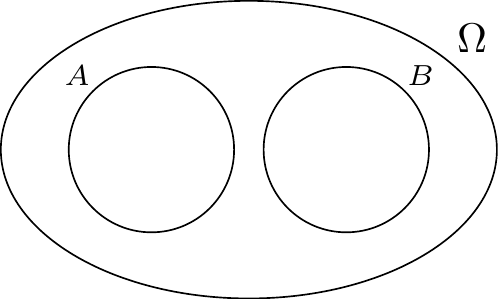
When two events have an empty intersection (i.e., they share no outcomes) we refer to them as disjoint or mutually exclusive.
Definition A.3 (Disjoint/mutually exclusive events) Events \(A\) and \(B\) are said to be disjoint when they share no outcomes, i.e., \(A \cap B = \emptyset\). More generally, a (potentially infinite) collection of events is said to be disjoint when no outcome belongs to more than one event in the collection. We also refer to a collection of disjoint events as mutually exclusive because no two of them can happen simultaneously.
As we will see in the coming chapters, recognizing when events are disjoint is very important. We give an example collection of disjoint events below.
Example A.4 (Mutually exclusive events) The events \(E_1^c \cap E_2 \cap E_3\) (first baby returned incorrectly and second and third babies returned correctly), \(E_1 \cap E_2^c \cap E_3\) (second baby returned incorrectly and first and third babies returned correctly), and \(E_1 \cap E_2 \cap E_3^c\) (third baby returned incorrectly and first and second babies returned correctly) are mutually exclusive. From the verbal description of the events, it is clear that they cannot share any outcomes. Any one of the events requires incorrectly returning a baby that is returned correctly in the others, so no two of them can happen at the same time.
Union
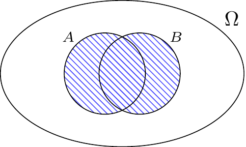
Next we introduce the union of two events \(A\) and \(B\), which is the event that at least one of \(A\) and \(B\) happens.
Definition A.4 (Union of two events) The union of events \(A\) and \(B\), denoted by \(A \cup B\), is the event that consists of any outcomes that are in at least one of \(A\) or \(B\). Colloquially, we refer to the event \(A \cup B\) as \(A \or B\).
Example A.5 (At least one of first two babies returned correctly) The event \(E_1 \cup E_2\) is the event that at least one of the first two babies is returned to their biological parents. It is made up of outcomes \(\omega = (\omega_1, \dots, \omega_n)\) where either \(\omega_1= 1\) or \(\omega_2=2\) (or both \(\omega_1= 1\) and \(\omega_2=2\)).
Like with intersections, we are often interested in the union of more than two events.
Definition A.5 (Union of many events) The union of a finite collection \(A_1, \dots, A_n\) of events (resp. an infinite collection \(A_1, A_2, \dots\) of events), denoted by \(\bigcup_{i=1}^n A_i\) or \(A_1 \cup \dots A_n\) (resp. \(\bigcup_{i=1}^{\infty} A_i\) or \(A_1 \cup A_2 \cup \dots\)), is the the event consisting of outcomes that are in at least one of the \(A_i\).
Example A.6 (At least one baby returned correctly) The event \(\bigcup_{i=1}^n E_i\) is the event that at least one of the babies is returned to their biological parents. It is made up of outcomes \(\omega = (\omega_1, \dots, \omega_n)\) where \(\omega_i = i\) for at least one \(i \in \{1, \dots, n\}\).
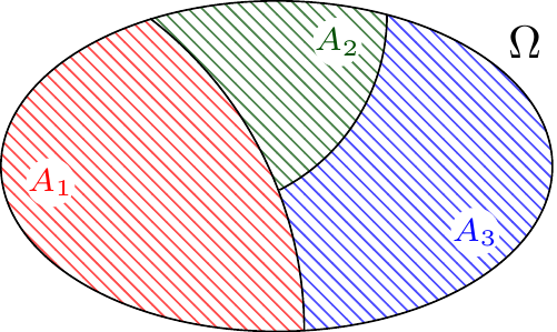
When we take the union of disjoint or mutually exclusive events, we sometimes call it a disjoint union. If a disjoint union of sets makes up the entire sample space, we say that those sets partition the sample space.
Definition A.6 (Partition) If \(A_1, \dots, A_n\) are disjoint events whose union is the whole sample space \(\Omega\) (i.e., \(\bigcup_{i=1}^n A_i = \Omega\)), then we say that the \(A_1, \dots, A_n\) are a partition of \(\Omega\).
Partitions will play an important role in Chapter 7 when we discuss the total law of probability.
Complement
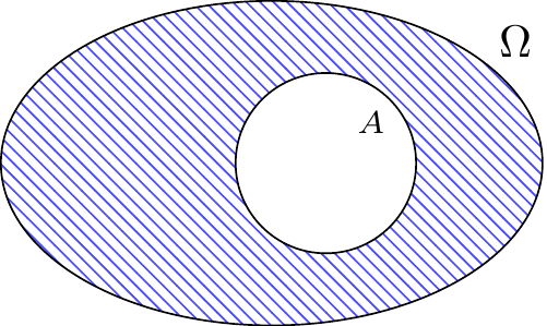
Lastly we define the complement of an event \(A\), which is the event that happens whenever \(A\) doesn’t.
Definition A.7 (Complement of an event) The complement of an event \(A\), denoted by \(A^c\), is the event consisting of outcomes that are not in \(A\). Colloquially, we refer to the event \(A\) as \(\not A\).
An event \(A\) and it’s complement \(A^c\) always partition the sample space. We give an example of this below and ask you to prove the more general claim as part of Exercise A.1.
Example A.7 (Partitioning on the first baby) Consider the event \(E_1\) that the first baby is returned correctly, which consists of all outcomes \(\omega = (\omega_1, \dots, \omega_n)\) with \(\omega_1= 1\). It’s complement \(E_1^c\) is the event that the first baby is returned incorrectly, which consists of all the outcomes \(\omega = (\omega_1, \dots, \omega_n)\) with \(\omega_1 \neq 1\). It’s clear that \(E_1\) and \(E_1^c\) are disjoint since an outcome \(\omega\) cannot have both \(\omega_1= 1\) and \(\omega_1 \neq 1\). Furthermore, since every outcome \(\omega\) must have either \(\omega_1=1\) or \(\omega_1 \neq 1\), every outcome must belong to either \(E_1\) or \(E_1^c\). Thus \(E_1 \cup E_1^c\) is a disjoint union that makes up the whole sample space, and \(E_1\) and \(E_1^c\) are therefore a partition of the sample space.
Countable and Uncountable Infinities
In closing, we briefly discuss the difference between countable and uncountable infinities. This is a subtle distinction, but one that is crucial in probability theory.
Definition A.8 (Countable and uncountable) An infinite collection of items is called countable if the items can be enumerated in a list. Conversely, if an infinite collection of items cannot be ennumerated in a list, it is called uncountable.
Example A.8 gives a few examples of both countable and uncountable infinities.
Example A.8 (Countable and uncountable infinities) An obvious example of a countably infinite collection of items is the natural numbers \(\mathbb{N} = \{1, 2, 3, \dots\}\). As written, we see that they are already enumerated in a list. The set of integers \(\mathbb{Z}\) is also countable. To see this, consider the list \[0, 1, -1, 2, -2, 3, -3, \dots\] In Exercise A.3, we ask you to argue that the rational numbers \(\mathbb{Q}\) (the set of all fractions) are also countable.
A classic example of an uncountably infinite collection of items is the set of infinite binary strings. To show that this collection is uncountable, we must prove that it cannot be enumerated in a list. For the interested reader, we show how do this via Cantor’s diagonlization argument.
Suppose for the sake of contraction that we could enumerate all infinite binary strings in a list:
\[\begin{matrix} \textbf{1.} & 0 & 1 & 0 & 1 & 0 & \dots \\
\textbf{2.} & 1 & 1 & 0 & 1 & 1 & \dots \\
\textbf{3.} & 1 & 1 & 0 & 0 & 0 & \dots \\
\textbf{4.} & 0 & 0 & 1 & 0 & 1 & \dots \\
\textbf{5.} & 1 & 1 & 1 & 1 & 0 & \dots \\
\vdots & \vdots & \vdots & \vdots & \vdots & \vdots & \ddots
\end{matrix}\]
Consider the infinite binary string whose \(i\)th entry matches that of the \(i\)th binary string in our list (i.e., it is given by the diagonal of our list). In our example, this string is \(01000\dots\). Make a new string from this one by flipping every \(0\) to a \(1\) and \(1\) to a \(0\). In our example, we get \(10111 \dots\). Since we’ve enumerated all infinite binary strings, this new string must be the \(j\)th string in our list for some positive integer \(j\). But, by how we’ve constructed this new string, its \(j\)th entry cannot match that of the \(j\)th string in our list, and therefore we have a contradiction.
In Exercise A.3, we ask you to use the same argument to show that \([0, 1]\), the set of real numbers between zero and one, is also uncountable. As a consequence, sets like the real line \(\mathbb{R}\) and the \(xy\)-plane \(\mathbb{R}^2\) are uncountable as well.
Exercises
Exercise A.1 Coming Soon!
Exercise A.2 Coming Soon!
Exercise A.3 Coming Soon!