In Chapter 13, we calculated conditional and marginal distributions from the joint distribution \(f_{X,Y}(x, y)\) of two random variables.
However, in many situations, the conditional distribution is known but not the joint distribution. The next example illustrates such a situation.
Example 16.1 (Corned Beef at the Food Truck) The number of customers \(N\) that purchase from a food truck at lunchtime follows a \(\text{Poisson}(\mu=\mean)\) distribution. About \(\textcolor{blue}{30\%}\) of customers order its signature corned beef sandwich, independently of other customers. Let \(X\) be the number of corned beef sandwiches they sell at lunchtime.
In this example, we know:
the marginal distribution of \(N\): \[ N \sim \text{Poisson}(\mu=\mean), \]
the conditional distribution of \(X\), given \(N\): \[ X \mid \{ N = n \} \sim \text{Binomial}(n, p=\prob). \]
but we do not know the joint distribution of \(X\) and \(N\), nor the marginal distribution of \(X\).
The food truck wants to know the (marginal) distribution of \(X\) so that they know how much corned beef to prepare. To find the marginal distribution, we can first find the joint distribution: \[\begin{align*}
f_{N, X}(n, x) &= f_N(n) \cdot f_{X \mid N}(x \mid n) \\
&= e^{-\mean} \frac{\mean^n}{n!} \cdot \frac{n!}{x! (n-x)!} (\prob)^x (1 - \prob)^{n-x}; & 0 \leq n < \infty, 0 \leq x \leq n
\end{align*}\]
and sum over \(n\) to get the marginal distribution of \(X\): \[\begin{align*}
f_X(x) &= \sum_n f_{N, X}(n, x) \\
&= \sum_{n=x}^\infty e^{-\mean} \frac{\mean^n}{n!} \cdot \frac{n!}{x! (n-x)!} (\prob)^x (1 - \prob)^{n-x} & (\text{probability is $0$ for $n < x$}) \\
&= e^{-\mean \cdot \prob} \frac{(\mean \cdot \prob)^x}{x!} \sum_{n=x}^\infty e^{-\mean (1 - \prob)} \frac{(\mean (1 - \prob))^{n-x}}{(n-x)!} & (\text{regroup terms}) \\
&= e^{-\mean \cdot \prob} \frac{(\mean \cdot \prob)^x}{x!} \underbrace{\sum_{m=0}^\infty e^{-\mean(1 - \prob)} \frac{(\mean(1 - \prob))^{m}}{m!}}_{=1} & (\text{substitute } m = n - x)\\
&= e^{-\mean \cdot \prob} \frac{(\mean \cdot \prob)^x}{x!}.
\end{align*}\]
In the last line, we used the fact that the expression inside the sum is a \(\text{Poisson}(\mu=\mean(1 - \prob))\) pmf. When we sum any pmf over all of its possible values, it is equal to \(1\).
The last step is to recognize the final expression for \(f_X(x)\) as the pmf of a Poisson random variable. In particular, \[X \sim \text{Poisson}(\mu=\mean \cdot \prob).\]
The algebra in Example 16.1 was tricky, but the idea was not. To obtain the marginal distribution of \(X\), we:
multiplied the distribution of \(N\) by the conditional distribution of \(X \mid N\) to get the joint distribution of \(N\) and \(X\)\[ f_{N, X}(n, x) = f_N(n) f_{X \mid N}(x \mid n) \]
summed the joint distribution over the values of \(N\) to get the distribution of \(X\). \[ f_X(x) = \sum_n f_{N, X}(n, x) \]
We can express this recipe as a single formula: \[ f_X(x) = \sum_n f_N(n) f_{X \mid N}(x \mid n). \tag{16.1}\] In fact, Equation 16.1 is none other than the Law of Total Probability! To see this, write each pmf in terms of the corresponding probability: \[ P(X = x) = \sum_n P(N = n) P(X = x \mid N = n). \tag{16.2}\] Since the sets \(A_n = \{ N = n \}\) form a partition of the sample space, Equation 16.2 is just a restatement of Theorem 7.1.
16.1 Law of Total Expectation
How many corned beef sandwiches should the food truck expect to sell at lunchtime? Since we already showed in Example 16.1 that \(X\) follows a \(\text{Poisson}(\mu=\mean \cdot \prob)\) distribution, and we know the expected value of a Poisson, the answer is: \[ \text{E}\!\left[ X \right] = \mu = \mean \cdot \prob = 25.56. \] But determining the (marginal) distribution of \(X\) was a lot of work! And in most situations, the marginal distribution may not be familiar, and may even be intractable to calculate.
Can \(\text{E}\!\left[ X \right]\) be calculated without first finding the distribution of \(X\)? The answer, surprisingly, is yes. The Law of Total Expectation, which is the natural extension of the Law of Total Probability (Equation 16.2) to expected values, says that \[
\text{E}\!\left[ X \right] = \sum_n P(N = n) \text{E}\!\left[ X \mid N = n \right].
\tag{16.3}\]
In words, it says that the overall expectation \(\text{E}\!\left[ X \right]\) can be calculated by:
first calculating the conditional expectations \(\text{E}\!\left[ X \mid N = n \right]\); and
weighting them by the probabilities of \(N\).
We will define the notation \(\text{E}\!\left[ X \mid N = n \right]\) in Definition 16.1 and prove the Law of Total Expectation in Theorem 16.1. But we will first apply it to two examples.
Example 16.2 (Corned Beef Expectations) How many corned beef sandwiches should the food truck expect to sell?
Since the conditional distribution \(X \mid N = n\) is binomial, we know that \[ \text{E}\!\left[ X \mid N = n \right] = np = n(\prob). \] Substituting this into the Law of Total Expectation (Equation 16.3), the expected number of corned beef sandwiches is \[\begin{align*}
\text{E}\!\left[ X \right] &= \sum_{n=0}^\infty e^{-\mean} \frac{(\mean)^n}{n!} \cdot n(\prob) \\
&= (\prob) \underbrace{\sum_{n=0}^\infty n \cdot e^{-\mean} \frac{(\mean)^n}{n!}}_{\text{E}\!\left[ N \right] = \mean} \\
&= 25.56.
\end{align*}\]
Notice how much simpler it is to calculate the expectation \(\text{E}\!\left[ X \right]\), compared with the distribution of \(X\) in Example 16.1. This illustrates the power of the Law of Total Expectation!
The next example applies the Law of Total Expectation to craps.
Example 16.3 (Expected Rolls in Craps) On average, how long does a round of craps last? Let’s determine the expected number of rolls in a round of craps.
Let \(X\) be the number of rolls after the come-out roll. The distribution of \(X\) is complicated. But the distribution of \(X\) is simple if we condition on the value of the come-out roll.
If the come-out roll is 2, 3, 7, 11, 12, then the round ends and \(X = 0\).
Otherwise, the come-out roll determines the point, and the number of remaining rolls \(X\) is a \(\Geom(p)\) random variable, where \(p\) depends on the point.
For example, if the point is 4, then the round ends when either a 4 or a 7 is rolled, so \(p = 9 / 36\).
But if the point is 9, then the round ends when either a 9 or a 7 is rolled, so \(p = 10/36\).
The outcome of the come-out roll is a random variable \(N\). Let’s calculate the conditional expectation \(\text{E}\!\left[ X \mid N = n \right]\) for different values of the come-out roll. We use the fact that the expected value of a \(\Geom(p)\) random variable is \(1 / p\). (We derived this previously using algebra, but it is also possible to derive this using conditional expectation. See Example 16.4.)
Come-Out Roll \(n\)
Distribution of \(X | N = n\)
\(\text{E}\!\left[ X | N = n \right]\)
2
\(0\)
\(0\)
3
\(0\)
\(0\)
4
\(\Geom(p=9/36)\)
\(36/9\)
5
\(\Geom(p=10/36)\)
\(36/10\)
6
\(\Geom(p=11/36)\)
\(36/11\)
7
\(0\)
\(0\)
8
\(\Geom(p=11/36)\)
\(36/11\)
9
\(\Geom(p=10/36)\)
\(36/10\)
10
\(\Geom(p=9/36)\)
\(36/9\)
11
\(0\)
\(0\)
12
\(0\)
\(0\)
Now, we can use the Law of Total Expectation to calculate \(\text{E}\!\left[ X \right]\). \[
\begin{align*}
\text{E}\!\left[ X \right] &= \sum_n P(N = n) \text{E}\!\left[ X \mid N = n \right] \\
&= P(N = 2) \underbrace{\text{E}\!\left[ X \mid N = 2 \right]}_0 + P(N = 3) \underbrace{\text{E}\!\left[ X \mid N = 3 \right]}_0 + \underbrace{P(N = 4)}_{3/36} \underbrace{\text{E}\!\left[ X \mid N = 4 \right]}_{36/9} + \cdots.
\end{align*}
\] This sum is rather tedious to calculate by hand, so we use R to finish the calculation.
From R, we see that \(\text{E}\!\left[ X \right] = 2.3758\).
The total number of rolls in the round includes the come-out roll, so it can be represented by the random variable \(1 + X\). Its expected value is \[ \text{E}\!\left[ 1 + X \right] = 1 + \text{E}\!\left[ X \right] = 3.3758. \]
16.2 Definitions and Proofs
To prove the Law of Total Expectation, we first need to define the conditional expectation \(\text{E}\!\left[ X \mid N = n \right]\). The definition is intuitive, as evidenced by the fact that we calculated it in the examples above before even defining it formally.
Definition 16.1 (Conditional Expectation Given an Event) The expectation of \(X\), conditional on an event \(A\), is defined as:
\[
\begin{align*}
\text{E}\!\left[ X \mid A \right] &\overset{\text{def}}{=} \sum_x x P(X = x \mid A) \\
&= \sum_x x f_{X \mid A}(x)
\end{align*}
\tag{16.4}\]
That is, instead of weighting the possible values of \(X\) by the probabilities of \(X\), we weight by its probabilities conditional on \(A\). These probabilities together comprise a (conditional) pmf \(f_{X \mid A}(x)\).
To define conditional expectations like \(\text{E}\!\left[ X \mid N = n \right]\), we simply condition on the event \(A = \{ N = n \}\) in Definition 16.1: \[
\begin{align*}
\text{E}\!\left[ X \mid N=n \right] &= \sum_x x P(X = x \mid N=n) \\
&= \sum_x x f_{X \mid N}(x \mid n).
\end{align*}
\tag{16.5}\]
Now, armed with Equation 16.5, we can state and prove the Law of Total Expectation.
Theorem 16.1 (Law of Total Expectation)\[ \text{E}\!\left[ X \right] = \sum_n P(N = n) \text{E}\!\left[ X \mid N = n \right]. \]
Proof
The proof follows by expanding \(\text{E}\!\left[ X \mid N = n \right]\) using its definition Equation 16.5 and rearranging the sums.
\[\begin{align*}
\sum_n P(N = n) \text{E}\!\left[ X \mid N=n \right] &= \sum_n P(N = n) \sum_x x P(X = x \mid N = n) \\
&= \sum_x x \underbrace{\sum_n P(N = n) P(X = x \mid N = n)}_{P(X = x)} \\
&= \text{E}\!\left[ X \right]
\end{align*}\]
We previously derived the expected value of a \(\Geom(p)\) random variable in Example 9.7. Now, we will demonstrate a much simpler derivation using the Law of Total Expectation.
Example 16.4 (Geometric Expectation using the Law of Total Expectation) Let \(X\) be a \(\Geom(p)\) random variable. What is \(\text{E}\!\left[ X \right]\)?
Let \(N\) be the outcome of the first Bernoulli trial. If \(N = 1\), then \(X = 1\). But if \(N = 0\), the number of remaining trials is again a \(\Geom(p)\) random variable.
In other words,
\(\text{E}\!\left[ X \mid N = 1 \right] = 1\)
\(\text{E}\!\left[ X \mid N = 0 \right] = 1 + \text{E}\!\left[ X \right]\), since we have used up \(1\) trial already and the remaining number of trials is again \(\Geom(p)\), with the same expectation.
By the Law of Total Expectation (Equation 16.3), we have the expression: \[
\begin{aligned}
\text{E}\!\left[ X \right] &= P(N = 0) \text{E}\!\left[ X \mid N = 0 \right] + P(N = 1) \text{E}\!\left[ X \mid N = 1 \right] \\
&= (1 - p) (1 + \text{E}\!\left[ X \right]) + p(1).
\end{aligned}
\]
Solving for \(\text{E}\!\left[ X \right]\), we obtain: \[ \text{E}\!\left[ X \right] = \frac{1}{p}. \]
Notice how we were able to obtain \(\text{E}\!\left[ X \mid N = 0 \right]\) by intuition and reasoning, rather than calculating it using Equation 16.4. This is typical of the situations where the Law of Total Expectation is most helpful.
Example 16.5 (Expected tosses until HH and HT) Hopefully, Equation 5.8 is deeply ingrained in your mind by now, and you know that we are equally likely to toss HH and HT with a fair coin.
Now, suppose we toss a fair coin repeatedly. Let \(X\) be the number of tosses until we see the sequence HT. Let \(Y\) be the number of tosses until we see the sequence HH (i.e., two heads in a row). How do \(\text{E}\!\left[ X \right]\) and \(\text{E}\!\left[ Y \right]\) compare?
Surprisingly, they are not the same! To see why, we calculate each using the Law of Total Expectation.
Let \(I_1\) be the indicator that the first toss is heads. First, we condition on the first toss, noting that
If the first toss is tails, then \(\text{E}\!\left[ X \mid I_1 = 0 \right] = 1 + \text{E}\!\left[ X \right]\), since the first toss was useless and we are effectively starting over.
If the first toss is heads, then we may continue to toss heads, but we will observe HT as soon as a tails is tossed. In other words, the remaining number of tosses is a \(\Geom(p = 1/2)\) random variable, so \(\text{E}\!\left[ X \mid I_1 = 1 \right] = 1 + \frac{1}{1 / 2} = 3\).
By the Law of Total Expectation, \[
\begin{align}
\text{E}\!\left[ X \right] &= P(I_1 = 0) \text{E}\!\left[ X \mid I_1 = 0 \right] + P(I_1 = 1) \text{E}\!\left[ X \mid I_1 = 1 \right] \\
&= \frac{1}{2} (1 + \text{E}\!\left[ X \right]) + \frac{1}{2} (3).
\end{align}
\] Solving for \(\text{E}\!\left[ X \right]\), we obtain \[
\text{E}\!\left[ X \right] = 4.
\]
To calculate \(\text{E}\!\left[ Y \right]\) requires two applications of the Law of Total Expectation. As before, we condition on the first toss, noting that \(\text{E}\!\left[ Y \mid I_1 = 0 \right] = 1 + \text{E}\!\left[ Y \right]\), since we have used up \(1\) toss and are no closer to seeing HH. Therefore, \[
\begin{align}
\text{E}\!\left[ Y \right] &= P(I_1 = 0) \text{E}\!\left[ Y \mid I_1 = 0 \right] + P(I_1 = 1) \text{E}\!\left[ Y \mid I_1 = 1 \right] \\
&= \frac{1}{2} (1 + \text{E}\!\left[ Y \right]) + \frac{1}{2} \text{E}\!\left[ Y \mid I_1 = 1 \right].
\end{align}
\tag{16.6}\]
However, we need to use the Law of Total Expectation again to calculate \(\text{E}\!\left[ Y \mid I_1 = 1 \right]\), conditioning also on the second toss. Let \(I_2\) be the indicator that the second toss is heads. Then,
\(\text{E}\!\left[ Y \mid I_1 = 1, I_2 = 0 \right] = 2 + \text{E}\!\left[ Y \right]\), since we are back where we started after \(2\) tosses.
\(\text{E}\!\left[ Y \mid I_1 = 1, I_2 = 1 \right] = 2\), since \(\{ I_1 = 1, I_2 = 1 \}\) implies that we have observed HH after \(2\) tosses.
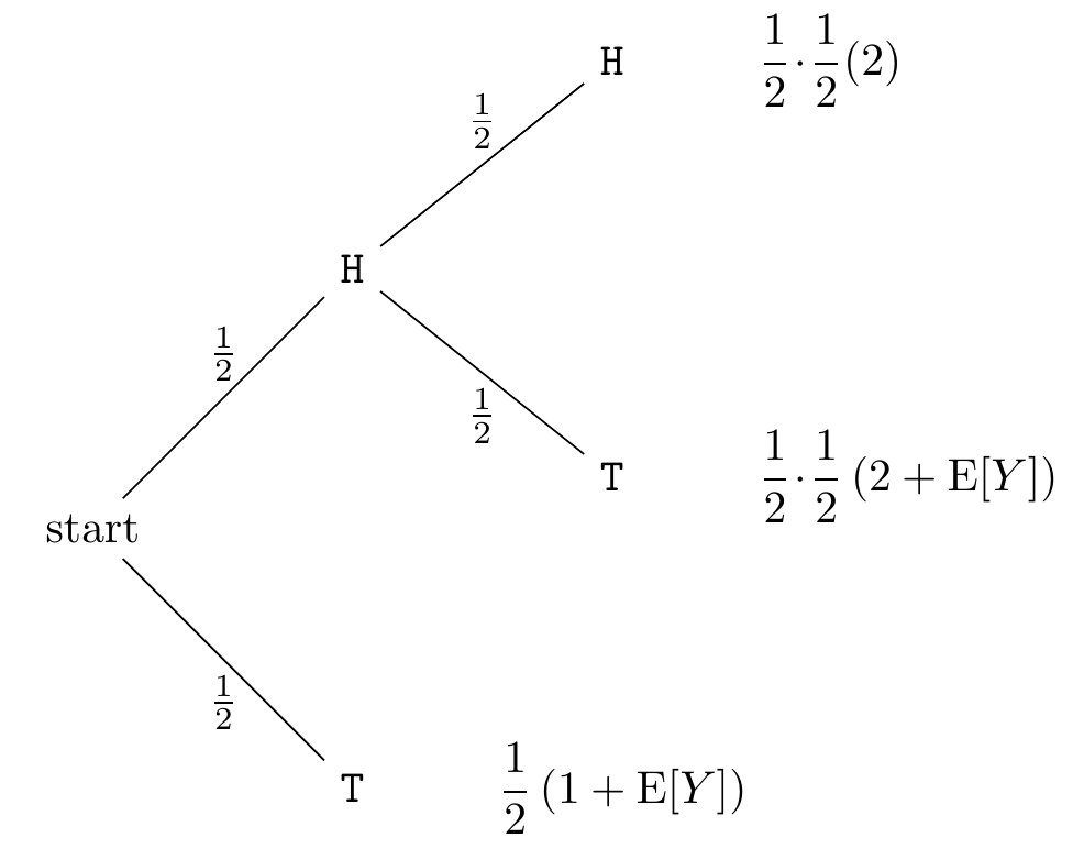
Now, we can plug this into Equation 16.6 and obtain \[
\begin{align}
\text{E}\!\left[ Y \right] &= \frac{1}{2} (1 + \text{E}\!\left[ Y \right]) + \frac{1}{2} \left(\frac{1}{2} (2 + \text{E}\!\left[ Y \right]) + \frac{1}{2} (2)\right).
\end{align}
\]
Solving this equation for \(\text{E}\!\left[ Y \right]\), we obtain \[
\text{E}\!\left[ Y \right] = 6.
\]
On average, it takes longer to observe HH than HT.
When there are multiple levels of conditioning, as in the calculation of \(\text{E}\!\left[ Y \right]\), it can be helpful to draw a probability tree (like we did in Example 5.4) to keep track of the different terms. In the tree below, the value calculated at each leaf is the contribution to the total expected value from that leaf.
16.3 Exercises
Exercise 16.1 (Noisy Channel) A stream of bits is being transmitted over a noisy channel. Each bit has a 1% chance of being corrupted, independently of any other bit. Let \(X\) be the number of bits that are transmitted until the first corruption.
Interpret \(\text{E}\!\left[ X \mid X > 10 \right]\) in the context of this problem.
Calculate \(\text{E}\!\left[ X \mid X > 10 \right]\).
Exercise 16.2 (Time until TTH and THT) A fair coin is tossed repeatedly.
Let \(X\) be the number of tosses until the sequence TTH first appears. What is \(\text{E}\!\left[ X \right]\)? Hint: Condition on the outcome of the first toss, and use Theorem 16.1.
Let \(Y\) be the number of tosses until the sequence THT first appears. What is \(\text{E}\!\left[ Y \right]\)?
Exercise 16.3 (Time until \(r\) heads in a row) Let \(X\) be the number of tosses of a coin (with probability \(p\) of landing heads) until you observe \(r\) consecutive heads (i.e., \(r\) heads in a row). Note that this is different from a negative binomial random variable, which is the number of tosses until you observe \(r\) total heads, not necessarily consecutive.
Calculate \(\text{E}\!\left[ X \right]\) in terms of \(r\) and \(p\), and compare it with the expectation of the corresponding negative binomial distribution. Does your answer make sense?
Exercise 16.4 (Die Game) You play the following game. You roll a fair, six-sided die. You can either take the amount on that die (in dollars) or roll the die again and take whatever amount comes up the second time (in dollars).
What is your optimal strategy? (In other words, when should you take the first roll, and when should you take the option to roll again?) How much money would you expect to win by playing this optimal strategy?
Now suppose that you have the option to roll the die a third time if you are unhappy with the outcome of the second roll. What is your optimal strategy now, and how much money would you expect to win with this strategy?