6 Independence

We opened Chapter 5 with a roulette example. We discussed how the relevant probability for a gambler who is considering entering the action after nine consecutive reds is \[ P(\text{10th spin is red}\ |\ \text{first 9 spins are red}), \] rather than the joint probability \[ P(\text{all 10 spins are red}). \]

Now that we have the tools to calculate conditional probabilities, let’s compute the probability above: \[ \begin{align*} P(\text{10th spin is red}\ &|\ \text{first 9 spins are red}) \\ &= \frac{P(\{\text{first 9 spins are red}\} \cap \{ \text{10th spin is red}\})}{P(\text{first 9 spins are red}) } \\ &= \frac{P(\text{all 10 spins are red})}{P(\text{first 9 spins are red}) } \\ &= \frac{ 18^{10}/38^{10} }{18^{9}/38^{9} } \\ &= \frac{18}{38}. \end{align*} \]

The probability that the 10th spin is red remains unchanged, as if we had no information about the previous spins. That is, \[ P(\text{10th spin is red}\ |\ \text{first 9 spins are red} ) = P(\text{10th spin is red}). \tag{6.1}\]

When the result of one event gives no information of the result of another, the two events are said to be independent. In this case, we say that the 10th spin is independent of the previous spins.

Nevertheless, Equation 6.1 might seem counterintuitive. Because ten reds in a row are extremely unlikely, many believe that the wheel should be “due” for a black after nine consecutive reds. This erroneous belief is known as the gambler’s fallacy.

6.1 Independence and its Properties

We formalize the above ideas in the following definition.

Definition 6.1 (Independence of two events) Two events $A$ and $B$ with positive probability are independent if either \[ P(A|B) = P(A) \] or \[ P(B|A) = P(B). \tag{6.2}\]

These two conditions are equivalent when $P(A) > 0$ and $P(B) > 0$. Otherwise, this would not be a valid definition.

To see why, note that the multiplication rule (Corollary 5.1) says \[P(A \cap B) = P(A)P(B|A) = P(B)P(A|B).\]

Now, if we assume the first condition, $P(A | B) = P(A)$, then the second equality above simplifies to \[ P(A) P(B | A) = P(B) P(A). \] Canceling $P(A)$ from both sides (which is legal because we assumed $P(A) > 0$), we obtain $P(B|A) = P(B)$, which is the second condition.

The proof that the second condition implies the first is similar.

While independence may be intuitively clear in simple cases like successive spins of a roulette wheel, other siations require us to check independence using Definition 6.1.

Example 6.1 (Betting on red and even) Suppose you make two bets, one on red and another on even, on a single spin of the roulette wheel. Are the two bets independent?

On a roulette wheel (Figure 1.5), there are $18$ red numbers and $18$ even numbers (0 and 00 do not count as even), but only $8$ numbers that are both red and even. Therefore: \[ \begin{align*} &P(\text{red}\ |\ \text{even} ) & \\ &= \frac{P(\text{red and even}) }{P(\text{even}) } \\ &= \frac{ 8/38 }{ 18/38 }\\ &= \frac{8}{18}. \end{align*} \] But this is not equal to $P(\text{red}) = \frac{18}{38}$, so red and even are not independent.

An equivalent characterization of independence comes from the multiplication rule (Corollary 5.1): two events are independent when the probability of both happening is equal to the product of their individual probabilities. It is usually easier to check independence using this characterization.

Proposition 6.1 (Independence of two events) Two events $A$ and $B$ with positive probability are independent if and only if \[ P(A \cap B) = P(A)P(B). \tag{6.3}\]

Probability zero events

When either $A$ or $B$ has zero probability, then both the left and right hand side of Equation 6.3 are zero. Because of this, probability zero events are considered to be independent of all other events.

Proof

Because the statement is an “if and only if” statement, we must show both directions. For both directions, we will use the multiplication rule (Corollary 5.1), which says \[P(A \cap B) = P(A)P(B|A). \tag{6.4}\]

[$\Rightarrow$] “Only if” direction:

Suppose that $A$ and $B$ are independent, so $P(B | A) = P(B)$. Substituting this into Equation 6.4, we obtain \[ P(A \cap B) = P(A) P(B), \] as we wanted to show.
[$\Leftarrow$] “If” direction:

Suppose that $P(A \cap B) = P(A) P(B)$. Substituting this into Equation 6.4, we obtain \[P(A) P(B) = P(A) P(B | A).\] Dividing both sides by $P(A)$ shows that $P(B) = P(B | A)$, which implies that $A$ and $B$ are independent.

We can use Proposition 6.1 to re-analyze Example 6.1.

Example 6.2 (Betting on red and even, revisited) We revisit Example 6.1, where we wanted to know if red and even in roulette are independent. Since

\[ P(\text{red and even}) = \frac{8}{38} \neq \frac{18}{38} \cdot \frac{18}{38} = P(\text{red})P(\text{even}), \] the two events cannot be independent.

Independence is also an important concept in genetics. Its meaning in genetics derives from its meaning in probability, as we show in the next example. This example also illustrates how Proposition 6.1 can be used to calculate probabilities.

Example 6.3 (Mendel’s Law of Independent Assortment) In Example 1.6, we learned that albinism is caused by a mutation in the OCA2 gene on chromosome 15. Each person has two copies of this gene, called alleles, which come in one of two versions:

$A$: the version without the mutation
$a$: the mutated version that can cause albinism

A person only exhibits albinism if both copies of the gene are the mutated version (i.e., they have genetic makeup $aa$).

Now, suppose we are also interested in the MC1R gene on chromosome 16, which influences whether a person has freckles. Like OCA2, MC1R has two alleles:

$B$: the version without the mutation
$b$: the mutated version that causes freckles

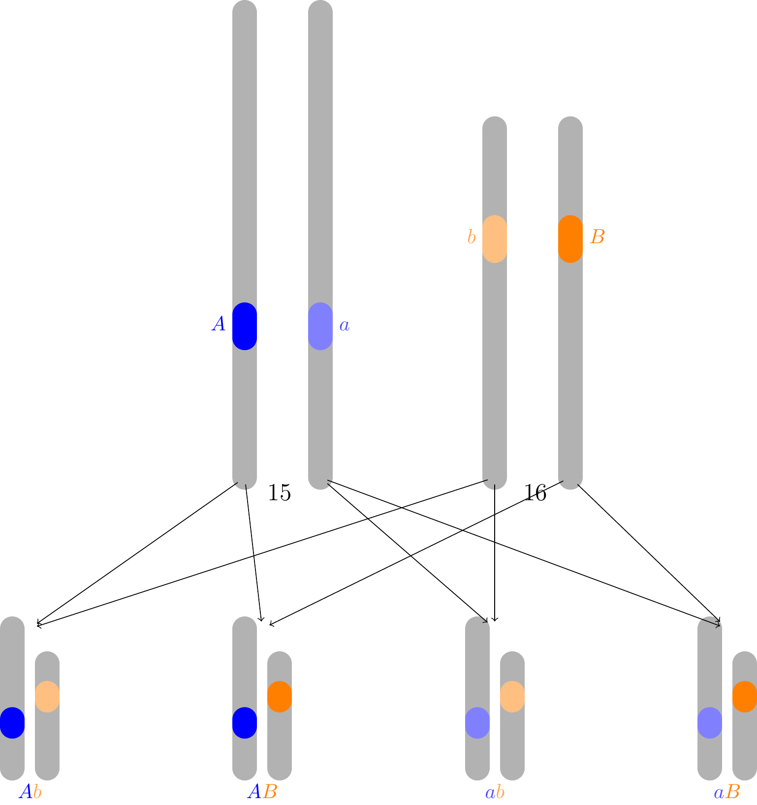
Mendel’s Law of Independent Assortment states that the two genes are inherited independently. (This is true because OCA2 and MC1R are on different chromosomes, although Mendel did not know this.) For example, suppose that both parents are carriers of the two traits (i.e., both parents have genetic makeup $AaBb$). Using Proposition 6.1 again, along with our earlier result, tells us that the probability of the child being albino and having freckles is

\[P(\text{child is } aabb ) = P(\text{child is } aa) P(\text{child is } bb) = \frac{1}{4} \cdot \frac{1}{4} = \frac{1}{16}.\]

Although the chances are small, there is a non-zero probability that two non-albino, non-freckled parents could have an albino child with freckles!

In many real world problems, we do not just work with two independent events, but rather a collection of many independent events. As Definition 6.2 explains, a collection of events is independent when knowing that a sub-collection of them occurred does not change the probability of any other event in the collection.

Definition 6.2 (Independence of many events) A (possibly infinite) collection of positive probability events $A_1, A_2, \dots$ is independent if the probability of any one of them happening does not change, given that some other finite sub-collection of them happened.

More concretely, for any two events,

\[ \begin{aligned} P(A_i| A_j) &= P(A_i) & i &\neq j, \end{aligned} \tag{6.5}\] and for any three events, \[ \begin{aligned} P(A_i| A_j, A_k) &= P(A_i) & i&\neq j \neq k, \end{aligned} \tag{6.6}\] and for any four events, \[ \begin{aligned} P(A_i| A_j, A_k, A_{\ell}) &= P(A_i) & i \neq j \neq k \neq \ell, \end{aligned} \tag{6.7}\]

and so on.

There is a similar characterization of independence in terms of multiplication, analogous to Proposition 6.1, which is often more useful.

Theorem 6.1 (Independence of many events) A (possibly infinite) collection of positive probability events $A_1, A_2, \dots$ is independent if and only if the probability of any finite sub-collection equals the product of the probabilities of the individual events in that sub-collection. That is, for any two events,

\[ \begin{aligned} P(A_i \cap A_j) &= P(A_i)P(A_j) & i &\neq j, \end{aligned} \tag{6.8}\]

and for any three events,

\[ \begin{aligned} P(A_i \cap A_j \cap A_k) &= P(A_i)P(A_j)P(A_k) & i &\neq j \neq k, \end{aligned} \tag{6.9}\]

and for any four events,

\[ \begin{aligned} P(A_i \cap A_j \cap A_k \cap A_\ell) &= P(A_i)P(A_j)P(A_k) P(A_\ell) & i &\neq j \neq k \neq \ell, \end{aligned} \tag{6.10}\]

and so on.

Probability zero events

For the same reason as in Proposition 6.1, any collection that contains an event with a probability of zero is considered to be independent.

Proof

Because the statement is an “if and only if” statement, we must show both directions. For both directions, we will use the general multiplication rule (Theorem 5.1), which says \[P(A_1 \cap A_2 \cap \dots \cap A_n) = P(A_1) P(A_2 | A_1) P(A_3 | A_1, A_2) \dots P(A_n| A_1, \dots A_{n-1}). \tag{6.11}\]

[$\Rightarrow$] “Only if” direction:

Suppose that the events are independent, meaning that the conditional probabilities satisfy Equation 6.5, Equation 6.6, and so on. Now, for any sub-collection, we can apply Equation 6.11 to obtain \[ \begin{align*} P(A_{i_1} \cap A_{i_2} \cap \dots \cap A_{i_n}) &= P(A_{i_1}) P(A_{i_2}|A_{i_1}) \dots P(A_{i_n}|A_{i_1}, A_{i_2}, \dots, A_{i_n}) \\ &= P(A_{i_1}) P(A_{i_2}) \dots P(A_{i_n}), \end{align*} \] where we used the assumption of independence in the last step. This shows that the probabilities multiply.
[$\Leftarrow$] “If” direction:

Suppose that the probabilities multiply, as in Equation 6.8, Equation 6.9, and so on. Then Equation 6.5 holds by Proposition 6.1, and Equation 6.6 holds because \[ \begin{align*} P(A_i)P(A_j)P(A_k) &= P(A_i \cap A_j \cap A_k) & \text{(assumed factoring)}\\ &= P(A_i) P(A_j | A_i)P(A_k | A_i, A_j) & \text{(multiplication rule)} \\ &= P(A_i) P(A_j) P(A_k | A_i, A_j). & \text{(previous result)} \end{align*} \] Dividing both sides by $P(A_i)P(A_j)$, we get that $P(A_k | A_i, A_j) = P(A_k)$. Now, we can show that Equation 6.7 and so on hold by induction. This proves that the events are independent in the sense of Definition 6.2.

Verifying that many events are collectively independent can be tricky. For example, even if all pairs of events in a collection are independent, the collection may not be independent as a whole. We ask you to construct a counterexample in Exercise 6.5.

Although the properties of independent collections are hard to characterize formally, the important properties are intuitive. For instance, if $A_1, A_2, \dots$ is an independent collection, then new collections of events like $E_1 = A_1^c$, $E_2 = A_2 \cup A_3$, and $E_3 = A_4 \cap A_5$ will also be independent—provided that no $A_i$ appears in more than one of the $E_j$. A general proof of this property is quite technical and beyond the scope of this book, but Exercise 6.6 invites you to check some particular instances of this fact.

6.2 Examples

Now, we work through several examples that use independence.

Example 6.4 (Cardano’s problem revisited) How many rolls of a fair die are needed to have a probability of at least $.5$ of rolling a six?

Let $A_i$ be the event that the $i$th roll is not a six. Since dice rolls are independent, $A_1, A_2, \dots$ are independent. Therefore, the probability of rolling a six in $n$ rolls is

\[ \begin{align*} P(\text{at least one six}) &= 1 - P(\text{no sixes}) & \text{(complement rule)}\\ &= 1 - P(A_1, \dots, A_n) & \text{(same event)}\\ &= 1 - P(A_1) \times \dots \times P(A_n) & \text{(independence)}\\ &= 1- \underbrace{\frac{5}{6} \times \dots \times \frac{5}{6}}_{n \text{ times}} & \text{(plug in probabilities)}\\ &= 1 - \left(\frac{5}{6}\right)^n \end{align*} \]

This agrees with our earlier answer from Example 4.1. As before, we can set this expression equal to $.5$ and solve for $n$ to see that $n \geq 4$.

By assuming independence, we can often obtain more precise answers to questions. In the next example, we re-analyze Example 4.5 with the added assumption of independence.

Example 6.5 (Quality control for medical devices revisited) Suppose, as in Example 4.5, we are manufacturing batches of $n=50$ medical devices. If each device we make has some failure probability $p$, how low does $p$ need to be to ensure that no devices fail with probability at least $99\%$?

We will assume that failures are due to one-off mishaps on the assembly line that have nothing to do with each other—that is, the failures of different devices are independent. Let $A_i$ be the event that the $i$th device fails. Then, the events $A_1, \dots, A_n$ are independent, as are their complements $A_1^c, \dots, A_n^c$. Therefore:

\[ \begin{align*} P(\text{no device fails}) &= P(A_1^c, \dots, A_{50}^c) \\ &= P(A_1^c) \times \dots \times P(A_{50}^c) & \text{(independence)}\\ &= (1-p)^{50} & \text{(earlier computation)} \end{align*} \]

Now, we want this probability to be at least $.99$. Solving for $p$, we obtain \[ p \leq 1 - (0.99)^{1/50} \approx .000201,\] which gives slightly more leeway than the worst-case analysis in Example 4.5, which required $p \leq .0002$. However, the difference is small, showing that the worst-case analysis was not so far off after all.

Next, we show how independence can be invoked intuitively to simplify calculations.

Example 6.6 (Winning a pass-line bet for a specific come-out roll) Suppose that in a round of craps (Example 1.9), the point has been set at five. What is the probability the shooter wins the round? That is, what is the probability that they roll a five again before rolling a seven?

Each time the shooter rolls the die, the result is either a five, a seven, or something else. If it is something else, then the shooter keeps rolling. Because the rolls are independent, the past rolls should not influence the current roll. Therefore, the probability that they win is the same as the probability that they roll a five, given that the round ends on the current roll. That is, \[ \begin{align*} P(\text{roll a five} &| \text{roll a five or a seven}) &\\ &= \frac{P(\text{roll a five})}{P(\text{roll a five or seven})} & \text{(definition of conditional probability)}\\ &= \frac{P(\text{roll a five})}{P(\text{roll a five} + \text{roll a seven})} & \text{(Axiom 3) }\\ &= \frac{4/36}{4/36 + 6/36} \\ &= \frac{4}{10}. \end{align*} \]

Notice how we appealed to independence to justify restricting our attention to the current roll. However, to prove this rigorously, we have to consider all of the rolls after the come-out roll.

Rigorous computation of the win probability

To compute the probability that the shooter wins, we calculate \[ \begin{align} P(\text{shooter wins}) &= P\left( \bigcup_{n=1}^\infty \{ \text{shooter wins on $n$th roll} \} \right) \\ &= \sum_{n=1}^\infty P(\text{shooter wins on $n$th roll}), \end{align} \] where the second equality follows from Axiom 3, since the events are mutually exclusive.

Now, let $A_i$ be the event that the $i$th roll is a five, $B_i$ the event that the $i$th roll is a seven, and $E_i = A_i \cup B_i$ the event that the round ends on the $i$th roll. Then, \[ \begin{align} P(\text{shooter wins on $n$th roll}) &= P(E_1^c, E_2^c, \dots, A_n) \\ &= P(E_1^c) P(E_2^c) \dots P(A_n) \\ &= \left(1 - \frac{10}{36}\right)^{n-1} \frac{4}{36}. \end{align} \]

Substituting this into the expression above, we obtain \[ \begin{align} P(\text{shooter wins}) &= \sum_{n=1}^\infty \left(1 - \frac{10}{36}\right)^{n-1} \frac{4}{36} \\ &= \frac{4}{36} \frac{1}{1 - (1 - \frac{10}{36})} & \text{(geometric series)} \\ &= \frac{4}{10}. \end{align} \]

Notice that the probability function $P$ above was really a conditional probability function (Proposition 5.1), since it was conditional on the event that the come-out roll is a five. We can repeat the above argument for different come-out rolls to obtain the following table of conditional probabilities.

$i$	$P(\text{win} \| \text{come-out roll is } i)$
2	$0$
3	$0$
4	$\frac{3}{9}$
5	$\frac{4}{10}$
6	$\frac{5}{11}$
7	$1$
8	$\frac{5}{11}$
9	$\frac{4}{10}$
10	$\frac{3}{9}$
11	$1$
12	$0$

Finally, we issue a cautionary tale about assuming independence.

Example 6.7 (Sally Clark case) An Englishwoman named Sally Clark experienced two back-to-back tragedies: in 1996, her first son died of sudden infant death syndrome (SIDS), and in 1998, her second son died under similar circumstances. She was arrested shortly afterwards and charged with murder.

At the trial, the pediatrician Roy Meadow testified that the probability of one child dying of SIDS was $1 / 8543$, so the probability of two children dying of SIDS was \[ P(\text{1st child suffers SIDS}) \cdot P(\text{2nd child suffers SIDS}) = \frac{1}{8543} \cdot \frac{1}{8543} \approx \frac{1}{73 \text{ million}}. \] On the basis of this testimony, Clark was convicted of murdering her two sons.

However, the Royal Statistical Society pointed out that Meadow’s calculation assumed independence, which was not justified for SIDS.

There may well be unknown genetic or environmental factors that predispose families to SIDS, so that a second case within the family becomes much more likely than would be a case in another, apparently similar, family.” (Green 2002)

In other words, the Royal Statistical Society argued that \[ P(\text{2nd child suffers SIDS}\ |\ \text{1st child suffers SIDS}) > P(\text{2nd child suffers SIDS}), \] so it is inappropriate to multiply the individual probabilities as if they were independent.

On the basis of this argument, Clark’s conviction was overturned on appeal in 2003, after she had served over three years of her sentence. Her life was never the same after the false accusation, and she sadly died four years later of alcohol poisoning.

6.3 Conditional Independence

Sometimes events are independent, but only if we condition on some other event having happened. Such events are said to be conditionally independent.

Definition 6.3 (Conditional independence) We say that a collection of (potentially infinite) positive probability events $A_1, A_2, \dots$ are conditionally independent given $B$, if they are independent under the conditional probability function $\widetilde P(A) \overset{\text{def}}{=}P(A|B)$—that is, \[ \widetilde P(A_{i_1} \cap A_{i_2} \cap \dots \cap A_{i_n}) = \widetilde P(A_{i_1}) \widetilde P(A_{i_2}) \dots \widetilde P(A_{i_n}) \tag{6.12}\] for any finite subcollection of $n$ events.

Note that by Proposition 5.1, this is equivalent to
\[ P(A_{i_1} \cap A_{i_2} \cap \dots \cap A_{i_n} | B) = P(A_{i_1} | B) P(A_{i_2} | B) \dots P(A_{i_n} | B). \]

One common misconception is that conditional independence implies unconditional independence, or vice-versa. In fact, neither is true. The next example illustrates conditionally independent events that are not unconditionally independent. You will come up with an example of unconditionally independent events that are not conditionally independent in Exercise 6.7.

Example 6.8 (COVID-19 antigen testing with one nurse) Suppose we selected a random New York resident around the end of March 2020 and wanted to know if they had COVID-19. We send them to a pop-up testing site where a nurse is administering an antigen test. These tests can randomly give incorrect readings due to manufacturing error and/or improper administration. To account for the possibility of an incorrect reading, the nurse administers two tests.

Considering the following five events,

$C_1$: the first test reading is correct,
$C_2$: the second test reading is correct,
$T_1$: the first test comes back positive,
$T_2$: the second test comes back positive,
$I$: the person is infected with COVID-19,

answer the following questions:

Q: Is it reasonable to assume that $C_1$ and $C_2$ are independent?

A: Yes. It’s certainly possible that slip-ups in manufacturing or administration could be due to random, one-off incidences. If so, then the correctness of one test does not inform us at all about the correctness of the other.
Q: Is it reasonable to assume that $T_1$ and $T_2$ are independent?

A: No. If one of the tests comes back positive, that should suggest an increased chance that the person actually has COVID-19. In turn, it should be more likely that the other test will also be positive.
Q: Is it reasonable to assume that $C_1$ and $C_2$ are conditionally independent given $I$?

A: Yes. If slip-ups in administration or mistakes in manufacturing are due to random, one-off incidences, then the person having COVID-19 will not change the fact that the correctness of one test does not inform us about the correctness of the other.
Q: Is it reasonable to assume that $T_1$ and $T_2$ are conditionally independent given $I$?

A: Yes. Conditional on the person having COVID-19, a positive test is the same as a correct test. We have already discussed why the tests’ correctness could be conditionally independent given that the person has COVID-19.

The next example builds on Example 6.8, showing that conditional independence can behave in counterintuitive ways. For example, even if events are conditionally independent given $B$, they may not be conditionally independent given $B^c$.

Example 6.9 (COVID-19 antigen testing with multiple nurses) Recall the COVID-19 testing example from Example 6.8, but now suppose that there are three nurses at our pop-up testing site. Two of the three nurses are experts, and their tests come back with the correct reading much more often than the third nurse, who is inexperienced and often administers the test incorrectly. The selected resident waits in line and is randomly helped by whichever nurse frees up first. Let $N_1$ and $N_2$ be the event that one of the two expert nurses administer the tests and $N_3$ be the event that the inexperienced nurse does.

Recalling the events from Example 6.8, we ask and answer two questions:

Q: Is it reasonable to assume that $C_1$ and $C_2$ are conditionally independent given $N_1$?

A: Yes. Since the same expert nurse is administering both tests, this is like our setting in Example 6.8, and it is reasonable to think that correctness of one test has no influence on the correctness of the other.
Q: Is it reasonable to assume that $C_1$ and $C_2$ are conditionally independent given $N_1^c$?

A: No. Given $N_1^c$ we know that either the other expert nurse or the inexperienced nurse is administering the tests, but we are not sure which one. If the first test is correct, it is more likely that the experienced nurse is administering the tests, and the second test should therefore also be more likely to be correct. Therefore, conditional on $N_1^c$, the correctness of the tests is not independent.

These examples show that conditional independence is a subtle, often fragile property—one we should assume with caution and apply with care.

6.4 Exercises

Exercise 6.1 (Fair coin from an unfair one) Suppose you have a coin with a probability $p\neq .5$ of landing heads. How can you use this unfair coin to simulate a fair coin?

Here is one idea: flip the coin twice. If the two flips are the same, discard the tosses and try again. If the two flips are different, call “heads” if it was HT and “tails” if it was TH.

Show that this method simulates a fair coin.

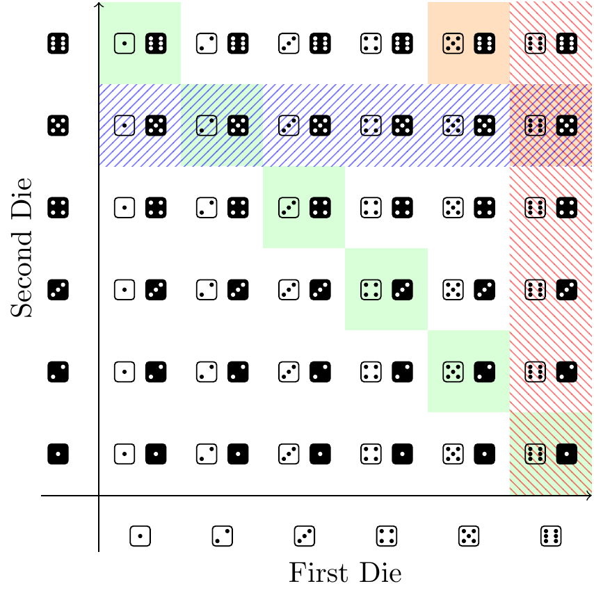
Exercise 6.2 (Rolling two dice and independence) Recall the experiment of rolling two fair dice, which has $36$ equally likely outcomes in its sample space:

Figure 6.1: Sample space for the experiment of rolling two six-sided dice. Outcomes in event $A$ highlighted in red (hatched), event $B$ in blue (hatched), event $C$ in orange (not hatched), and event $D$ in green (not hatched).

Considering the four events,

$A$: the first (white) die lands on $6$
$B$: the second (black) die lands on $5$
$C$: the rolled numbers sum to $11$
$D$: the rolled numbers sum to $7$

answer the following questions:

Are $A$ and $B$ independent? Is this what you expected?
Are $A$ and $C$ independent? Is this what you expected?
Are $A$ and $D$ independent? Is this what you expected?
Are $C$ and $D$ independent? Is this what you expected?

Exercise 6.3 Show that, if $A$ and $B$ are independent events, then

$A$ and $B^c$ are independent,
$A^c$ and $B$ are independent,
$A^c$ and $B^c$ are independent.

Hint

Once you do a., you should be able to immediately use it to imply b. and c.

Exercise 6.4 Recall the experiment of rolling two fair die from Exercise 6.2. What is the probability that first die does not land on $6$ and the sum of the dice is also not 7? Rather than counting, use the results from Exercise 6.2 and Exercise 6.3 to come up with your answer.

Exercise 6.5 Come up with a collection of events where all the pairs of events are independent, but the collection is not independent as a whole.

Hint

Use three events from Exercise 6.2.

Exercise 6.6 Suppose that $A_1, A_2, \dots$ is a collection of independent events. Show that

$A_1 \cap A_2$ and $A_3^c$ are independent
$A_1 \cup A_2$, $A_3 \cap A_4^c$, and $A_5$ is a collection of independent events.
$A_1, A_2^c, A_3, A_4^c, A_5, A_6^c, \dots$ is a collection of independent events.
$A_1$ and $A_1^c \cap A_2$ are not necessarily independent events.
$A_1, A_1 \cup A_2, A_1 \cup A_2 \cup A_3, \dots$ is not necessarily a collection of independent events.

Exercise 6.7 Show that there exist events $A$ and $B$ that are independent, but not conditionally independent given a third event $C$.

Hint

Use the events from Exercise 6.2.

Exercise 6.8 Suppose that $A$, $B$, $C$ are an independent collection of events and $C$ has positive probability. Show that $A$ and $B$ are conditionally independent given $C$.

\(i\)	\(P(\text{win} \| \text{come-out roll is } i)\)
2	\(0\)
3	\(0\)
4	\(\frac{3}{9}\)
5	\(\frac{4}{10}\)
6	\(\frac{5}{11}\)
7	\(1\)
8	\(\frac{5}{11}\)
9	\(\frac{4}{10}\)
10	\(\frac{3}{9}\)
11	\(1\)
12	\(0\)