In this chapter, we develop a measure of the strength of the relationship between two variables called covariance. It is based on \(\text{E}\!\left[ XY \right]\), which we learned to calculate in Section 14.3.
- First, when \(X\) and \(Y\) have “no” relationship—that is, they are independent—we know that \(\text{E}\!\left[ XY \right] = \text{E}\!\left[ X \right]\text{E}\!\left[ Y \right]\) from Theorem 14.3.
- But if \(X\) and \(Y\) tend to vary together (if one is large, the other is also), then their product \(XY\) will tend to be larger than under independence, so \(\text{E}\!\left[ XY \right] > \text{E}\!\left[ X \right] \text{E}\!\left[ Y \right]\).
- On the other hand, if \(X\) and \(Y\) tend to vary in opposite directions so that one is small when the other is large, then \(XY\) will tend to be smaller than under independence, so \(\text{E}\!\left[ XY \right] < \text{E}\!\left[ X \right] \text{E}\!\left[ Y \right]\).
In other words, when \(\text{E}\!\left[ XY \right]\) is larger (resp. smaller) than \(\text{E}\!\left[ X \right] \text{E}\!\left[ Y \right]\), it suggests a positive (resp. negative) association. The next definition takes independence as a baseline and is constructed to be zero when \(X\) and \(Y\) are independent. Therefore, its sign indicates the direction of the relationship between \(X\) and \(Y\).
Definition 15.1 (Covariance) Let \(X\) and \(Y\) be random variables. Then, the covariance between \(X\) and \(Y\) is \[
\text{Cov}\!\left[ X, Y \right] \overset{\text{def}}{=}\text{E}\!\left[ XY \right] - \text{E}\!\left[ X \right]\text{E}\!\left[ Y \right].
\tag{15.1}\]
Our definition of covariance differs from some books. See Exercise 15.1.
In some sense, the covariance measures how far two random variables are from independence, although it is not a perfect measure, as we will see in Example 15.3.
In the next example, we practice calculating and interpreting covariances.
Example 15.1 (Covariance between two genes) Recall Example 14.5, where there were two genes. \(X\) was defined to be the number of copies of the dominant \(A\) allele that a child inherits and \(Y\) was defined to be the number of copies of the dominant \(B\) allele. Since \(X\) and \(Y\) are both \(\textrm{Binomial}(n= 2, p= 1/2)\) random variables, \[
\text{E}\!\left[ X \right] = \text{E}\!\left[ Y \right] = 2\cdot \frac{1}{2} = 1.
\]
We will calculate \(\text{Cov}\!\left[ X, Y \right]\) under the three different models from Chapter 13. We already calculated \(\text{E}\!\left[ XY \right]\) under each model in Example 14.5.
If the two genes are on different chromosomes, then \(X\) and \(Y\) are independent, so \[ \text{Cov}\!\left[ X, Y \right] = 0 \tag{15.2}\] by definition, but we can also calculate it: \[
\text{Cov}\!\left[ X, Y \right] = \text{E}\!\left[ XY \right] - \text{E}\!\left[ X \right] \text{E}\!\left[ Y \right] = 1 - 1 = 0.
\]
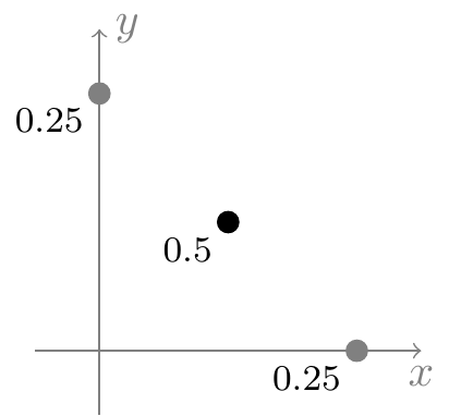
If the two genes are on the same chromosome, without recombination, then \[ \text{Cov}\!\left[ X, Y \right] = \text{E}\!\left[ XY \right] - \text{E}\!\left[ X \right] \text{E}\!\left[ Y \right] = 0.5 - 1 = -0.5. \tag{15.3}\] Notice that this covariance is negative, which makes sense because \(Y\) is low (\(Y = 0\)) precisely when \(X\) is high (\(X = 2\)), and vice versa, as shown in Figure 15.1.
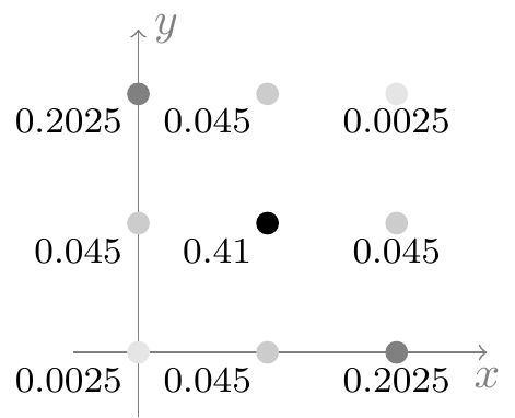
Finally, in the presence of recombination, the covariance is \[ \text{Cov}\!\left[ X, Y \right] = \text{E}\!\left[ XY \right] - \text{E}\!\left[ X \right] \text{E}\!\left[ Y \right] = 0.6 - 1 = -0.4. \tag{15.4}\] This covariance is still negative, but its magnitude is less than Equation 15.3, indicating that recombination weakens the negative relationship between \(X\) and \(Y\). This is apparent from Figure 15.2, since now outcomes like \(\{ X = 0, Y = 0 \}\) and \(\{ X=2, Y=2 \}\) are possible, but their probabilities are small, and the prevailing relationship is still negative.
Properties of Covariance
We can use the following properties to calculate many covariances without 2D LotUS (Theorem 14.1).
Proposition 15.1 (Properties of covariance) Let \(X, Y, Z\) be random variables and \(a\) be a constant. Then, the following are true.
- (Symmetry) \(\text{Cov}\!\left[ X, Y \right] = \text{Cov}\!\left[ Y, X \right]\).
- (Constants cannot covary) \(\text{Cov}\!\left[ a, Y \right] = 0\).
- (Multiplying by a constant) \(\text{Cov}\!\left[ a X, Y \right] = a \text{Cov}\!\left[ X, Y \right] = \text{Cov}\!\left[ X, a Y \right]\).
- (Distributive property) \(\text{Cov}\!\left[ X+Y, Z \right] = \text{Cov}\!\left[ X, Z \right] + \text{Cov}\!\left[ Y, Z \right]\) and \(\text{Cov}\!\left[ X, Y+Z \right] = \text{Cov}\!\left[ X, Y \right] + \text{Cov}\!\left[ X, Z \right]\).
Property 1 follows immediately from Equation 15.1.
To prove Property 2, we plug in \(a\) for \(X\): \[
\text{Cov}\!\left[ a, Y \right] \overset{\text{def}}{=}\text{E}\!\left[ aY \right] - \text{E}\!\left[ a \right]\text{E}\!\left[ Y \right] = a\text{E}\!\left[ Y \right] - a\text{E}\!\left[ Y \right] = 0.
\]
To prove Property 3, we plug in \(aX\) for \(X\): \[
\begin{aligned}
\text{Cov}\!\left[ aX, Y \right] &= \text{E}\!\left[ aXY \right] - \text{E}\!\left[ aX \right]\text{E}\!\left[ Y \right] \\
&= a\text{E}\!\left[ XY \right] - a\text{E}\!\left[ X \right]\text{E}\!\left[ Y \right] \\
&= a(\text{E}\!\left[ XY \right] - \text{E}\!\left[ X \right]\text{E}\!\left[ Y \right]) \\
&= a\text{Cov}\!\left[ X, Y \right].
\end{aligned}
\]
To prove Property 4, we plug in the random variables into Equation 15.1 and use properties of expectation, especially linearity. \[
\begin{aligned}
\text{Cov}\!\left[ X + Y, Z \right] &= \text{E}\!\left[ (X + Y)Z \right] - \text{E}\!\left[ X + Y \right]\text{E}\!\left[ Z \right] \\
&= \text{E}\!\left[ XZ + YZ \right] - (\text{E}\!\left[ X \right] + \text{E}\!\left[ Y \right])\text{E}\!\left[ Z \right] \\
&= \text{E}\!\left[ XZ \right] + \text{E}\!\left[ YZ \right] - \text{E}\!\left[ X \right]\text{E}\!\left[ Z \right] - \text{E}\!\left[ Y \right]\text{E}\!\left[ Z \right] \\
&= (\text{E}\!\left[ XZ \right] - \text{E}\!\left[ X \right]\text{E}\!\left[ Z \right]) + (\text{E}\!\left[ YZ \right] - \text{E}\!\left[ Y \right]\text{E}\!\left[ Z \right]) \\
&= \text{Cov}\!\left[ X, Z \right] + \text{Cov}\!\left[ Y, Z \right].
\end{aligned}
\]
The covariance is also intimately related to the variance. In fact, the variance is simply the covariance of a random variable with itself.
Proposition 15.2 (Relationship between variance and covariance) Let \(X\) be a random variable. Then, \[
\text{Var}\!\left[ X \right] = \text{Cov}\!\left[ X, X \right].
\]
Substituting \(X\) for \(Y\) in Definition 15.1, we obtain \[
\text{Cov}\!\left[ X, X \right] = \text{E}\!\left[ XX \right] - \text{E}\!\left[ X \right] \text{E}\!\left[ X \right] = \text{E}\!\left[ X^2 \right] - \text{E}\!\left[ X \right]^2,
\] but this is just the shortcut formula for variance (Proposition 11.2).
These properties often allow us to calculate covariances without using 2D LotUS. The next example revisits one of the calculations from Example 15.1.
Example 15.2 (Covariance between two genes without recombination) When the two genes are on the same chromosome, then in the absence of recombination, we saw in Example 13.2 that \(Y = 2 - X\).
By properties of covariance, \[
\begin{align}
\text{Cov}\!\left[ X, Y \right] &= \text{Cov}\!\left[ X, 2 - X \right] \\
&= \underbrace{\text{Cov}\!\left[ X, 2 \right]}_{0} - \underbrace{\text{Cov}\!\left[ X, X \right]}_{\text{Var}\!\left[ X \right]} \\
&= -\text{Var}\!\left[ X \right] \\
&= -2 \cdot \frac{1}{2} \left(1 - \frac{1}{2}\right) = -0.5,
\end{align}
\] where we used the formula for the variance of a binomial random variable (Proposition 11.3). This matches the answer that we obtained in Equation 15.3, but we did not need to calculate \(\text{E}\!\left[ XY \right]\) or use the joint PMF at all.
Now, as promised, we show that covariance is not necessarily a good measure of how far two random variables are from independence. Although independence implies zero covariance, two random variables can have zero covariance without being independent.
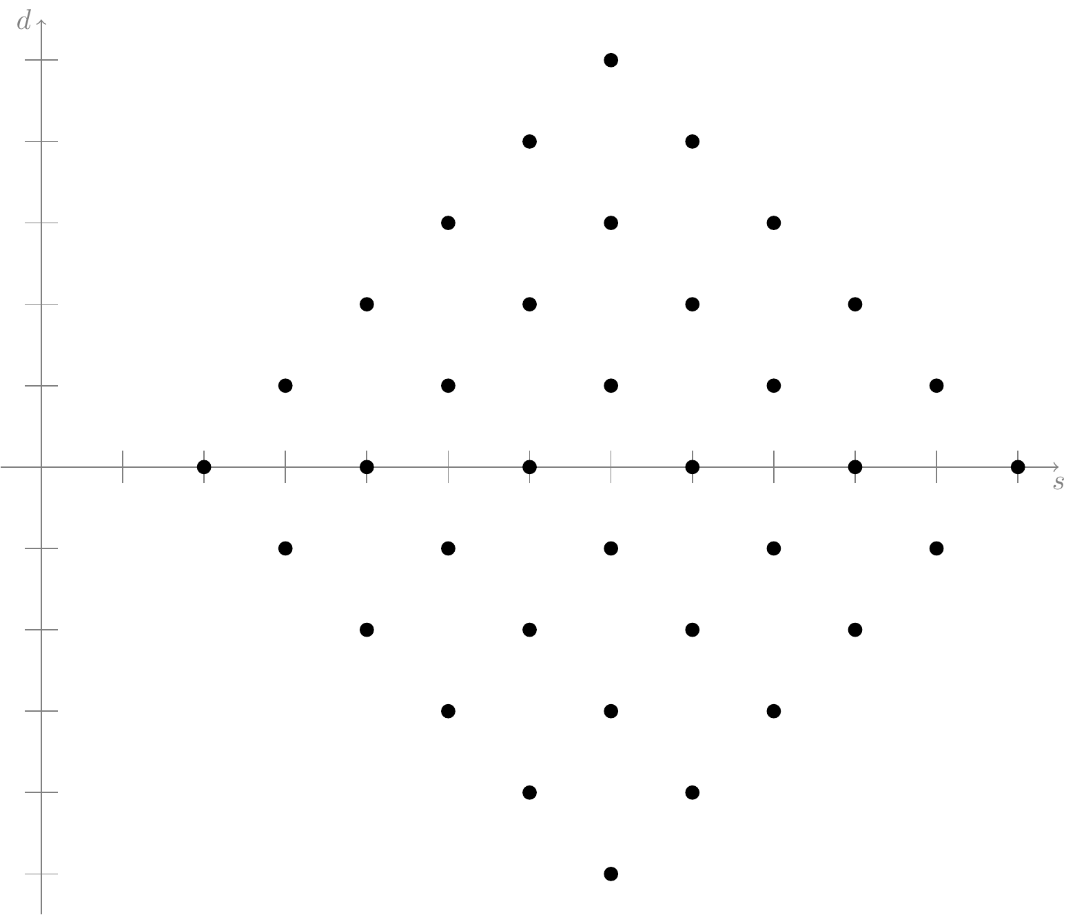
Example 15.3 (Sum and difference of die rolls) Suppose we roll two fair six-sided dice; let \(X\) be the outcome on the first die and \(Y\) be the outcome on the second die. Note that \(X\) and \(Y\) are independent, so \(\text{Cov}\!\left[ X, Y \right] = 0\).
Let \(S = X+Y\) be the sum and \(D = X-Y\) be the difference. Then, the covariance between \(S\) and \(D\) is \[\begin{align*}
\text{Cov}\!\left[ S, D \right] &= \text{Cov}\!\left[ X+Y, X-Y \right] \\
&= \text{Cov}\!\left[ X, X \right] - \text{Cov}\!\left[ X, Y \right] + \text{Cov}\!\left[ Y, X \right] - \text{Cov}\!\left[ Y, Y \right] \\
&= \text{Var}\!\left[ X \right] - \text{Var}\!\left[ Y \right] \\
&= 0.
\end{align*}\]
Notice that we did not even need to calculate the variance for a six-sided die, since \(X\) and \(Y\) have the same distribution and thus the same variance.
Although \(S\) and \(D\) have zero covariance, they are not independent. To see why, consider \(P(D = 0)\) and \(P(D = 0 \mid S = 12)\). If the two random variables were independent, these two probabilities would need to be equal.
- \(P(D = 0) = 6/36\), since a difference of \(0\) means that the two dice show the same number.
- \(P(D = 0 \mid S = 12) = 1\), since a sum of \(12\) implies that both dice showed a six, so \(D = 0\).
Since we have found a pair \((d, s)\) for which \(P(D = d \mid S = s) \neq P(D = d)\), \(D\) and \(S\) cannot be independent. (Per Definition 13.2, independence requires that equality holds for all \(d\) and \(s\).)
Figure 15.3 provides intuition about why the covariance is \(0\). Although \(S\) and \(D\) are not independent, they do not consistently vary in the same or opposite directions, which is why their covariance is neither positive nor negative.
Note that the \(\text{Cov}\!\left[ S,D, = \right] 0\) result did not require \(XD\) and \(Y\) to be independent; we only needed them to have the same variance.
The key takeaway from Example 15.3 is:
By Theorem 14.3, if \(X\) and \(Y\) are independent, then \(\text{Cov}\!\left[ X, Y \right] = 0\).
However, the converse is not true. It is possible for \(\text{Cov}\!\left[ X, Y \right] = 0\), even though \(X\) and \(Y\) are not independent, as Example 15.3 illustrates.
Using Covariance to Calculate Variances
Because of Proposition 15.2, we can use properties of covariance to calculate variances. In the next example, we compute variances using covariance to quantify the difference between two betting strategies.
Example 15.4 (Comparing roulette bets) Wanda brings $10 to a roulette table. She is deciding between the following ways to spend her $10:
- betting $1 on red in each of ten spins of the roulette wheel, or
- betting $10 on red in one spin of the roulette wheel.
How do these two strategies compare?
If we let \(W_1, W_2, \dots, W_{10}\) represent the profits from $1 bets (on red) on ten spins of the roulette wheel, then her total profits from the two options are
- \(W_1 + W_2 + \dots + W_{10}\), and
- \(10 W_1\).
Note that \(W_1, W_2, \dots, W_{10}\) are independent.
The two options have the same expectation, since \[
\text{E}\!\left[ W_1 + W_2 + \dots + W_{10} \right] = \text{E}\!\left[ W_1 \right] + \text{E}\!\left[ W_2 \right] + \dots + \text{E}\!\left[ W_{10} \right] = 10 \text{E}\!\left[ W_1 \right]
\] and \[
\text{E}\!\left[ 10 W_1 \right] = 10 \text{E}\!\left[ W_1 \right].
\]
However, their variances are very different. The first strategy has a variance of \[
\begin{align}
\text{Var}\!\left[ W_1 + W_2 + \dots + W_{10} \right] &= \text{Cov}\!\left[ W_1 + W_2 + \dots + W_{10}, W_1 + W_2 + \dots + W_{10} \right] \\
&= \sum_{k=1}^{10} \text{Cov}\!\left[ W_k, W_k \right] + \sum_{j\neq k} \underbrace{\text{Cov}\!\left[ W_j, W_k \right]}_{0} \\
&= 10 \text{Var}\!\left[ W_1 \right].
\end{align}
\]
The variance of the second strategy can be calculated using Proposition 11.4 or directly using properties of covariance: \[
\begin{align}
\text{Var}\!\left[ 10 W_1 \right] &= \text{Cov}\!\left[ 10 W_1, 10 W_1 \right] \\
&= 10^2 \text{Cov}\!\left[ W_1, W_1 \right] \\
&= 100 \text{Var}\!\left[ W_1 \right].
\end{align}
\]
On average, Wanda makes the same amount with either bet, but with a single $10 bet, she is putting all her eggs in one basket. She either wins big or loses big, which is why this option has the higher variance.
We could obtain numerical values by calculating \(\text{E}\!\left[ W_1 \right]\) and \(\text{Var}\!\left[ W_1 \right]\), but the result is true, no matter what their values are. This means that the same conclusion holds whenever the small bets are independent and identically distributed.
Finally, we use properties of covariance to provide simple derivations of the binomial and hypergeometric variances. Compare this next derivation with Proposition 11.3.
Example 15.5 (Binomial variance using covariance) Let \(X \sim \text{Binomial}(n,p)\). In Example 14.3, we wrote \[ X = I_1 + I_2 + \dots + I_n, \] where \(I_k\) is the indicator of heads on the \(k\)th toss, and we applied linearity of expectation to evaluate \(\text{E}\!\left[ X \right]\).
We can apply properties of covariance to the same decomposition in order to evaluate \(\text{Var}\!\left[ X \right]\).
\[\begin{align*}
\text{Var}\!\left[ X \right] &= \text{Cov}\!\left[ X, X \right] \\
&= \text{Cov}\!\left[ I_1 + \cdots + I_n, I_1 + \cdots + I_n \right] \\
&= \sum_k \underbrace{\text{Cov}\!\left[ I_k, I_k \right]}_{\text{Var}\!\left[ I_k \right]} + \sum_{j \neq k} \underbrace{\text{Cov}\!\left[ I_j, I_k \right]}_0 \\
&= \sum_{k=1}^n p(1-p) \\
&= np(1-p).
\end{align*}\]
In the third equality, we used independence of the coin tosses to conclude that \(\text{Cov}\!\left[ I_j, I_k \right] = 0\) for \(j \neq k\).
What about the hypergeometric variance? In Example 14.4, we argued that we could also represent a hypergeometric random variable using the same sum of indicator random variables, except that the indicators are no longer independent. This did not affect the expectation (because of linearity), but it does affect the variance.
Example 15.6 (Hypergeometric variance using covariance) Let \(Y \sim \text{Hypergeometric}(n, M, N)\). In Example 14.4, we expressed \(Y\) as a sum of indicator random variables, \[ Y = I_1 + I_2 + \dots + I_n, \] where \(I_k\) is \(1\) if the \(k\)th can sampled is defective.
If we apply properties of covariance to evaluate \(\text{Var}\!\left[ Y \right]\), as in Example 15.5,
\[\begin{align*}
\text{Var}\!\left[ Y \right] &= \text{Cov}\!\left[ Y, Y \right] \\
&= \text{Cov}\!\left[ I_1 + \cdots + I_n, I_1 + \cdots + I_n \right] \\
&= \sum_k \underbrace{\text{Cov}\!\left[ I_k, I_k \right]}_{\text{Var}\!\left[ I_k \right]} + \sum_{j \neq k} \text{Cov}\!\left[ I_j, I_k \right],
\end{align*}
\] we encounter a snag. The draws are not independent, so we cannot conclude that \(\text{Cov}\!\left[ I_j, I_k \right] = 0\) for \(j \neq k\). We need to calculate this covariance from Definition 15.1. Recalling that these random variables are Bernoulli random variables and are either \(0\) or \(1\),
\[
\begin{aligned}
\text{Cov}\!\left[ I_j, I_k \right] &= \text{E}\!\left[ I_jI_k \right] - \text{E}\!\left[ I_j \right]\text{E}\!\left[ I_k \right] \\
&= P(I_j = 1, I_k = 1) - P(I_j = 1) P(I_k = 1) \\
&= \frac{M}{N} \frac{M - 1}{N - 1} - \frac{M}{N} \frac{M}{N} \\
&= -\frac{M}{N} \frac{N - M}{N} \frac{1}{N - 1} \\
&= - \frac{M}{N} \left(1 - \frac{M}{N}\right) \frac{1}{N-1}
\end{aligned}
\] Notice that this covariance is negative. This makes sense because if we sample a defective can, that makes it less likely that we will sample another defective can. Therefore, \(I_j\) and \(I_k\) tend to move in opposite directions.
Now, substituting this covariance into the complete expression, we have
\[\begin{align*}
\text{Var}\!\left[ Y \right] &= \sum_k \frac{M}{N} \left(1 - \frac{M}{N}\right) - \sum_{j \neq k} \frac{M}{N} \left(1 - \frac{M}{N}\right) \frac{1}{N - 1} \\
&= n \frac{M}{N} \left(1 - \frac{M}{N}\right) - n (n - 1)\frac{M}{N} \left(1 - \frac{M}{N}\right) \frac{1}{N - 1} \\
&= n \frac{M}{N} \left(1 - \frac{M}{N}\right) \left(1 - \frac{n - 1}{N - 1} \right),
\end{align*}
\] which (after a bit of algebra) matches the expression we derived in Proposition 12.1.
Exercises
Exercise 15.1 (Alternative definition of covariance) Many books define covariance as \[
\text{Cov}\!\left[ X, Y \right] \overset{\text{def}}{=}\text{E}\!\left[ (X - \text{E}\!\left[ X \right])(Y - \text{E}\!\left[ Y \right]) \right]
\tag{15.5}\] instead of Equation 15.1.
We show that our definition implies Equation 15.5.
- Show that \(\text{Cov}\!\left[ X, Y \right] = \text{Cov}\!\left[ X - \text{E}\!\left[ X \right], Y - \text{E}\!\left[ Y \right] \right]\).
- Calculate \(\text{Cov}\!\left[ X - \text{E}\!\left[ X \right], Y - \text{E}\!\left[ Y \right] \right]\) using Definition 15.1 and simplify, establishing Equation 15.5.
Exercise 15.2 (Covariance of coin tosses) Consider the following scenarios:
- A fair coin is tossed 3 times. \(X\) is the number of heads and \(Y\) is the number of tails.
- A fair coin is tossed 4 times. \(X\) is the number of heads in the first 3 tosses and \(Y\) is the number of heads in the last 3 tosses.
- A fair coin is tossed 6 times. \(X\) is the number of heads in the first 3 tosses and \(Y\) is the number of heads in the last 3 tosses.
Calculate \(\text{Cov}\!\left[ X, Y \right]\) for each scenario. Do the signs make sense?
Hint: You can calculate the covariance using 2D LotUS or using properties of covariance.
Exercise 15.3 (Covariance between \(X\) and \(X^2\)) Let \(X\) be a discrete random variable that is symmetric around 0. That is, \(-X\) has the same PMF as \(X\).
Calculate \(\text{Cov}\!\left[ X, X^2 \right]\). Are \(X\) and \(X^2\) independent?
Exercise 15.4 (Covariance between spades and hearts in a poker hand) Suppose you are dealt a poker hand of \(5\) cards from a well-shuffled deck of cards. Let \(X\) be the number of spades in the hand, and let \(Y\) be the number of hearts in the hand. Calculate and interpret \(\text{Cov}\!\left[ X, Y \right]\).
(Hint: Although you derived the joint PMF of \(X\) and \(Y\) in Exercise 13.2, it is much easier to calculate the covariance by expressing \(X\) and \(Y\) as a sum of indicators.)
Exercise 15.5 (Variance of Happy Meals purchased) Let \(X\) be the total number of Happy Meals purchased in Exercise 14.6. Compute \(\text{Var}\!\left[ X \right]\).