4 Properties of Probability Functions

In Chapter 3, we defined a probability rigorously by specifying the axioms that a probability function $P$ must satisfy. In this chapter, we derive a few consequences of those axioms, which will enhance our toolset for computing probabilities.

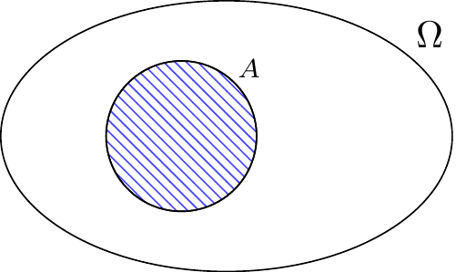
Throughout this chapter, we will illustrate sample spaces and events with diagrams like Figure 4.1.

Figure 4.1: In a sample space $\Omega$, an event $A$ marked in blue.

In Figure 4.1, the area of the event $A$, shaded in blue, represents the probability $P(A)$. Since Kolmogorov’s second axiom (see Definition 3.1) requires $P(\Omega) = 1$, we imagine that the area of the entire sample space is one. Therefore, $P(A)$ can be thought of as the proportion of the sample space that $A$ occupies.

4.1 Complement Rule

In many situations, the probability of an event is difficult to calculate directly, but the probability of its complement is straightforward. The complement rule relates the two probabilities.

Proposition 4.1 (Complement rule) For any event $A$,

\[P(A^c) = 1 - P(A).\]

Proof

Intuitively, the statement is true because, as Figure 4.2 shows, the sum of the areas covered by $A$ and $A^c$ is equal to the area covered by the sample space $\Omega$, which is $1$.

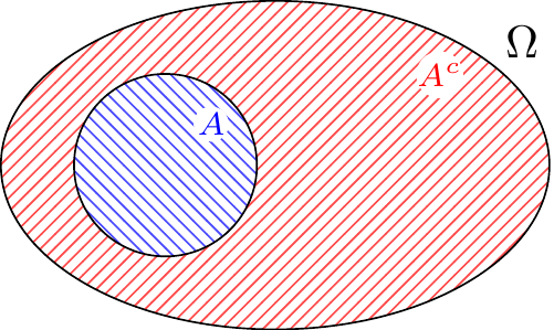
Figure 4.2: In a sample space $\Omega$, an event $A$ marked in blue and its complement $A^c$ marked in red.

To prove this formally, note that $A$ and $A^c$ are disjoint, and their union is $\Omega$.

Therefore, by Axiom 3 of Definition 3.1, \[ P(\Omega) = P(A \cup A^c) = P(A) + P(A^c), \] and by Axiom 2, $P(\Omega) = 1$. The result now follows by moving $P(A)$ to the other side.

We already used the complement rule implicitly when solving Cardano’s problem in Solution 2.1. The next example spells this out explicitly.

Example 4.1 (Revisiting Cardano’s problem) How many times do we need to roll a fair die to have at least a $1/2$ probability of seeing one or more sixes?

First, we determine the probability of rolling at least one six in $n$ rolls. It is not straightforward to count the number of ways of rolling at least one six. For example, perhaps the first roll was a six, or maybe the last roll was a six, or possibly both rolls were sixes.

The complement of this event is “no sixes in $n$ rolls.” It is much easier to count the number of ways of rolling no sixes; it simply means that one of the other $5$ sides was rolled $n$ times. \[ \begin{align} P(\text{at least one six in $n$ rolls}) &= 1 - P(\text{no sixes in $n$ rolls}) \\ &= 1 - \frac{5^n}{6^n}. \end{align} \]

To finish the problem, we simply need to solve for $n$ that makes this probability at least $1/2$: \[ \begin{align} 1 - \left(\frac{5}{6}\right)^n &\geq \frac{1}{2} \\ n &\geq \frac{\log(1/2)}{\log(5/6)} \approx 3.8, \end{align} \] so at least $n=4$ rolls are necessary.

Kolmogorov’s axioms (Definition 3.1) do not directly guarantee that probabilities have to be between zero and one. However, this is an immediate consequence of the complement rule.

Proposition 4.2 (Probabilities are between zero and one) For any event $A$,

\[0 \leq P(A) \leq 1.\]

Proof

Axiom 1 (see Definition 3.1) already guarantees that $P(A) \geq 0$ for any event $A$.

By the complement rule (Proposition 4.1), $P(A) = 1 - P(A^c)$. Since Axiom 1 implies $P(A^c) \geq 0$, it must also be the case that $P(A) \leq 1$.

4.2 Subset Rule

If a set $B$ is contained within another set $A$ (see Figure 4.3), then we say that $B$ is a subset of $A$, which we write as $B \subseteq A$. This means that whenever the event $B$ happens, the event $A$ also happens. The next result relates the probability of two events when one is a subset of another.

Proposition 4.3 (Subset rule) For any events $A$ and $B$ such that $B \subseteq A$, \[P(B) \leq P(A).\]

Proof

Intuitively, when $B$ is a subset of $A$ it cannot cover a larger portion of the sample space than $A$.

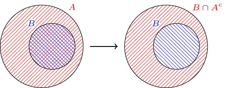
To prove this formally, we observe that if $B \subseteq A$, we can write $A$ as the disjoint union of $B$ and $A \cap B^c$.

Now, by Axiom 3 (see Definition 3.1), \[P(A) = P(B) + P(A \cap B^c). \] Since Axiom 1 (see Definition 3.1) guarantees that $P(A \cap B^c) \geq 0$, it must be the case that $P(A) \geq P(B)$.

Even though the subset rule seems obvious in the abstract, it is not always intuitive when applied to real world problems, as the next example shows.

Example 4.2 (Linda problem) The psychologists Amos Tversky and Daniel Kahneman presented subjects with the following scenario:

Linda is 31 years old, single, outspoken, and very bright. She majored in philosophy. As a student, she was deeply concerned with issues of discrimination and social justice, and also participated in anti-nuclear demonstrations.

They then asked which of the following was more probable:

Linda is a bank teller.
Linda is a bank teller and is active in the feminist movement.

They found that the majority of subjects chose the second option. However, by the subset rule, it is impossible for the second option to be more probable, even without any specific information about Linda.

To be precise, the event \[ \{ \text{Linda is a bank teller} \} \cap \{ \text{Linda is active in the feminist movement} \} \] is a subset of \[ \{ \text{Linda is a bank teller} \}, \] so by Proposition 4.3,

\[ P(\text{Linda is a bank teller and is active in the feminist movement}) \leq P(\text{Linda is a bank teller}). \]

This is true for any probability function $P$, so it holds even if Linda is very likely to be in the feminist movement. The erroneous belief that $P(A \cap B)$ can sometimes be larger than $P(A)$ is known as the conjunction fallacy. Kahneman (2011, chap. 15) discusses this example as well as others.

As another example, we can use Proposition 4.3 to establish that the probability of tossing the infinite sequence HHHHHHH... with a fair coin is zero.

Example 4.3 (Probability of tossing all heads) Recall the sample space from Example 3.11, which consisted of all infinite sequences of heads and tails. If we define \[ A_i \overset{\text{def}}{=}\{ \omega: \text{$\omega_i$ is heads} \}, \] then the event that all of the tosses are heads can be written as \[ \bigcap_{i=1}^\infty A_i. \]

To determine the probability of this event, we observe that it is a subset of the event that the first $n$ tosses are heads: \[ \bigcap_{i=1}^\infty A_i \subseteq \bigcap_{i=1}^n A_i. \] In Example 3.11, we discussed that the probability function $P$ assigns the probability \[ P\left( \bigcap_{i=1}^n A_i \right) = \frac{1}{2^n} \] to the latter event. Therefore, by the subset rule, \[ P\left(\bigcap_{i=1}^\infty A_i\right) \leq P\left(\bigcap_{i=1}^n A_i\right) = \frac{1}{2^n}. \] However, this inequality is true for any number of tosses $n$. Letting $n \to \infty$, we see that \[ P\left(\bigcap_{i=1}^\infty A_i\right) = 0. \tag{4.1}\] That is, the probability of tossing the sequence HHHHHH... must be zero.

In fact, the same argument shows that the event that any specific sequence $\omega$ of heads and tails shows up has zero probability. Perhaps this is not so surprising; there are so many possible sequences that the chance that any particular sequence, such as HHTHTTH..., shows up is infinitesimally small.

4.3 Properties of Unions

4.3.1 Union of Two Events

If two events are mututally exclusive, then we can calculate the probability of their union by simply adding their probablities (by Axiom 3 of Definition 3.1). What if they are not mutually exclusive? The next result provides a general way to calculate the probability of the union of two events.

Proposition 4.4 (Addition rule) For any events $A$ and $B$,

\[P(A \cup B) = P(A) + P(B) - P(A \cap B).\]

Proof

$P(A \cup B)$ is the total area covered by the two circles in Figure 4.4. Intuitively, we see that adding together $P(A)$ and $P(B)$ double-counts the area in their intersection. Subtracting $P(A\cap B)$ corrects for this overcounting. We formalize this argument below.

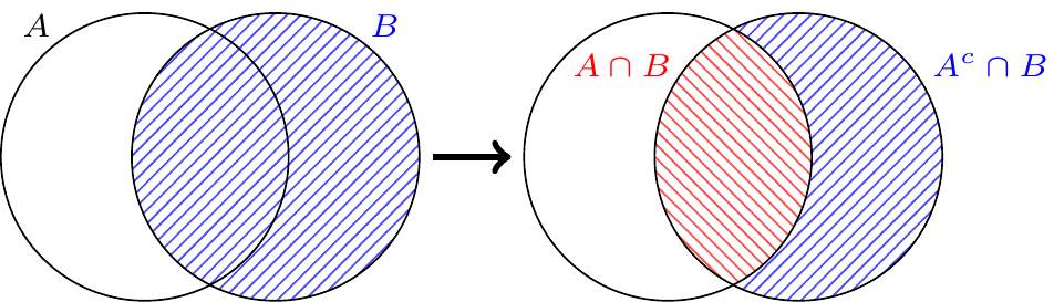
To make use of Axiom 3, we need to express $A \cup B$ as a union of sets that are disjoint. As illustrated below, $A \cup B$ can be written as the disjoint union of $A$ and $A^c \cap B$, the part of $B$ that is not in $A$.

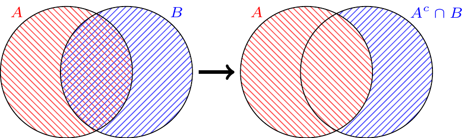
Figure 4.4: Visual proof that $A \cup B$ is the disjoint union of $A$ and $A^c \cap B$.

So by Axiom 3: \[P(A \cup B) = P(A \cup (A^c \cap B)) = P(A) + P(A^c \cap B).\]

To complete the proof, we need to show that $P(A^c \cap B) = P(B) - P(A \cap B)$. But again, we can write $B$ as the disjoint union of $A \cap B$, the part of $B$ that is in $A$, and $A^c \cap B$, the part of $B$ that is not in $A$:

Figure 4.5: Visual proof that $B$ is the disjoint union of $A \cap B$ and $A^c \cap B$.

By Axiom 3, $P(A \cap B) + P(A^c \cap B) = P(B)$. By moving $P(A \cap B)$ to the other side, we obtain the desired result.

The addition rule describes a fundamental relationship between $P(A)$, $P(B)$, $P(A \cap B)$, and $P(A \cup B)$. If we know or can compute three of these, we can find the fourth.

Example 4.4 (Winning at least one bet in roulette (revisited)) In Example 3.7, we considered the probability that a gambler who bets on “red” and “even” on one spin of the roulette wheel wins at least one of these bets. That is, if $A$ is the event that she wins the “red” bet and $B$ is the event that she wins the “even” bet, we want to know $P(A \cup B)$.

Previously, we calculated this probability by counting the number of outcomes in the union. However, we already know from Example 1.4 that \[ P(A) = P(B) = \frac{18}{38} \] and we showed in Example 3.4 that \[ P(A \cap B) = \frac{8}{38}. \]

Therefore, by the addition rule, we know that \[ P(A \cup B) = P(A) + P(B) - P(A \cap B) = \frac{18}{38} + \frac{18}{38} - \frac{8}{38} = \frac{28}{38}. \]

4.3.2 The Union Bound

Because $P(A \cap B) \geq 0$, the sum of the individual probabilities \[ P(A) + P(B) \] overestimates the probability of the union \[ P(A \cup B) = P(A) + P(B) - P(A \cap B). \] In other words, the sum of the individual probabilities is an upper bound for the probability of the union: \[ P(A \cup B) \leq P(A) + P(B). \]

This fact generalizes to the union of more than two events.

Proposition 4.5 (Union bound) For a collection of events $A_1, \dots, A_n$, \[ P \left( \bigcup_{i=1}^n A_i \right) \leq \sum_{i=1}^n P(A_i). \tag{4.2}\]

The union bound is also sometimes called Boole’s inequality.

Proof

This proof uses a technique called induction. Equation 4.2 is clearly true when $n=1$, in which case it reduces to $P(A_1) \leq P(A_1)$.

Next, we prove that if Equation 4.2 is true when $n = k$, then it is also true when $n = k+1$. That is, suppose we can assume that \[ P \left( \bigcup_{i=1}^k A_i \right) \leq \sum_{i=1}^k P(A_i). \tag{4.3}\] Equation 4.3 is called the inductive hypothesis. Armed with the inductive hypothesis, we try to show that Equation 4.2 also holds when $n = k+1$. \[ \begin{align} P \left( \bigcup_{i=1}^{k+1} A_i \right) &= P\left(\left( \bigcup_{i=1}^k A_i \right) \cup A_{k+1} \right) \\ &= P\left( \bigcup_{i=1}^k A_i \right) + P(A_{k+1}) - P\left( \left( \bigcup_{i=1}^k A_i \right) \cap A_{k+1} \right) & \text{(addition rule)} \\ &\leq \sum_{i=1}^k P(A_i) + P(A_{k+1}) - P\left( \left( \bigcup_{i=1}^k A_i \right) \cap A_{k+1} \right) & \text{(inductive hypothesis)} \\ &\leq \sum_{i=1}^k P(A_i) + P(A_{k+1}). & \text{(Axiom 1)} \end{align} \tag{4.4}\]

This is exactly what we wanted to show: the sum of the probabilities of $k+1$ events is an upper bound for the probability of their union.

Why does this argument establish Equation 4.2? Since we know that it is true for $n = 1$, Equation 4.4 implies that it must also be true when $n = 2$. But if it is true when $n = 2$, we can apply Equation 4.4 again to see that it must also be true when $n = 3$. And so on. The induction argument establishes that Equation 4.2 is true for any number of events $n$.

The union bound is useful for bounding probabilities of rare events.

Example 4.5 (Quality control for medical devices) A company manufactures medical devices in batches of 50. They want to ensure that, at least $99\%$ of the time, none of the devices in a batch fail. How reliable do they need to make each device in the batch? That is, how low does the failure probability $p$ for an individual device need to be?

They want to ensure that $P(\text{no device fails}) \geq .99$. By the complement rule (Proposition 4.1), this is true if \[ P(\text{some device fails}) \leq .01. \]

Since the event that some device fails can be written as a union of the events $F_i$ that the $i$th device fails, we can use the union bound to bound the probability of it happening:

\[ P(\text{some device fails}) = P \left(\bigcup_{i=1}^{50} F_i \right) \leq \sum_{i=1}^{50} P(F_i) = 50p \]

The company needs $50 p \leq .01$; in other words, $p \leq .01 / 50 = .0002$.

Is it necessary to have $p \leq .0002$? Technically, it is. If the failure events $F_i$ are mutually exclusive (i.e., no two devices in the same batch ever fail at the same time), then by Axiom 3 \[ P(\text{some device fails}) = P\left(\bigcup_{i=1}^{50} F_i \right) = \sum_{i=1}^{50} P(F_i) = 50p . \] In this case, if $p > .0002$, then $P(\text{some device fails}) > .01$ and $P(\text{no device fails}) < .99$.

Treating the failure events as mutually exclusive is unrealistic. In Chapter 6 we will refine this analysis by making realistic assumptions about the failures of the devices.

Although the union bound can be useful for rare events, it can produce unhelpful answers.

Example 4.6 (Secret Santa with the union bound) Recall Example 1.7, where four friends draw slips of paper to determine whom they will buy a gift for. What can we say about the probability of a “good draw,” where no one draws their own name?

First, we can use the complement rule: \[ P(\text{no one draws own name}) = 1 - P(\text{at least one person draws own name}). \]

Let $E_i$ denote the probability that friend $i$ draws their own name. Then we can write \[ P(\text{at least one person draws own name}) = P\left( \bigcup_{i=1}^4 E_i \right). \]

The union bound tells us that this probability is \[P \left(\bigcup_{i=1}^4 E_i\right) \leq \sum_{i=1}^4 P(E_i).\]

To calculate $P(E_i)$, we can count outcomes in the sample space as follows. There are $4!$ equally likely outcomes. If friend $i$ draws their own name, then there are $3!$ ways that the other three friends could draw names. Therefore, \[ P(A_i) = \frac{3!}{4!} = \frac{1}{4} \] for $i = 1, 2, 3, 4$. Alternatively, we could appeal to symmetry: each friend is drawing one of four slips at random, so the chance that they draw their own name must be $1/4$.

Therefore, the union bound says \[P \left(\bigcup_{i=1}^4 E_i\right) \leq \sum_{i=1}^4 \frac{1}{4} = 1.\]

Since we already know that probabilities cannot be greater than $1$ (see Proposition 4.2), this bound is useless!

The union bound also extends to (countably) infinite events $A_1, A_2, \dots$.

Proposition 4.6 (Union bound for infinitely many events) For a collection of events $A_1, A_2, \dots$, \[ P \left( \bigcup_{i=1}^\infty A_i \right) \leq \sum_{i=1}^\infty P(A_i). \tag{4.5}\]

4.3.3 Inclusion-Exclusion Principle

As we saw in Example 4.6, the union bound does not always yield helpful answers. Now, we discuss how to calculate the probability of a union exactly, although the method is not always easy to apply.

To build intuition for the general result, we first consider the union of three events. Conceptually we can think of the probability $P(A \cup B \cup C)$ as the area of the region covered by the three circles in Figure 4.6.

Figure 4.6: Three events $A$, $B$, and $C$.

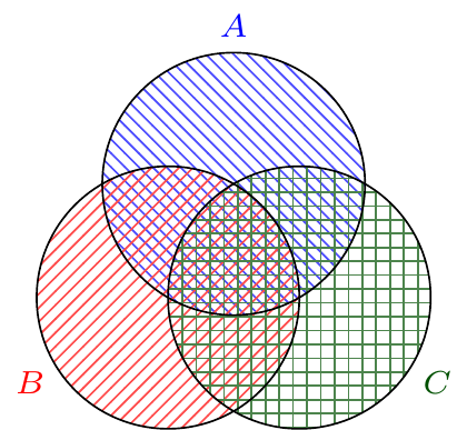
If we add together the areas of the circles $A$, $B$ and $C$, this will double-count the area in the intersections $A \cap B$, $B \cap C$, and $A \cap C$. We could try to adjust for this by subtracting off the probability of each intersection once:

\[P(A) + P(B) + P(C) - P(A \cap B) - P(B \cap C) - P(A \cap C). \]

However, now the area in the intersection $A \cap B \cap C$ has been added in three times by $P(A)$, $P(B)$, and $P(C)$ but also subtracted three times by $P(A \cap B)$, $P(B \cap C)$, and $P(A \cap C)$. Therefore, we have to add it back in once, yielding the formula

\[P(A \cup B \cup C) = P(A) + P(B) + P(C) - P(A \cap B) - P(B \cap C) - P(A \cap C) + P(A \cap B \cap C). \]

The inclusion-exclusion principle generalizes this result to the union of $n$ events.

Theorem 4.1 (Inclusion-exclusion principle) For a collection of events $A_1, \dots, A_n$,

\[ \begin{align*} P \left( \bigcup_{i=1}^n A_i \right) &= \sum_{i=1}^n P(A_i) - \sum_{1 \leq i < j \leq n } P(A_i \cap A_j) \\ &\qquad + \sum_{1 \leq i < j < k \leq n} P(A_i \cap A_j \cap A_k) - \dots + (-1)^{n+1} P(A_1 \cap \dots \cap A_n) \end{align*} \tag{4.6}\]

Proof

Equation 4.6 is notationally dense, so we break it down:

\[ \textcolor{orange}{\underbrace{\sum_{i=1}^n P(A_i)}_{(1)}} - \textcolor{magenta}{\underbrace{\sum_{1 \leq i < j \leq n } P(A_i \cap A_j)}_{(2)}} + \textcolor{purple}{\underbrace{\sum_{1 \leq i < j < k \leq n} P(A_i \cap A_j \cap A_k)}_{(3)}} - \dots + (-1)^{n+1} \textcolor{brown}{\underbrace{P(A_1 \cap \dots \cap A_n)}_{(n)}}.\]

Since each of the terms $\textcolor{orange}{(1)}, \textcolor{magenta}{(2)}, \textcolor{purple}{(3)}, \dots, \textcolor{brown}{(n)}$ is a sum, we can regard the expression as an alternating sum of sums. It is alternating in the sense that we start with the sum $\textcolor{orange}{(1)}$, then subtract the sum $\textcolor{magenta}{(2)}$, then add the sum $\textcolor{purple}{(3)}$, and so on. The $m$th term is essentially a sum over the different ways one can choose $m$ events from the $n$ events in the union. As such, Proposition 2.3 tells us that the $m$th term is the sum of ${{n}\choose{m}}$ different probabilities; the last term $\textcolor{brown}{(n)}$ is the sum of just ${{n}\choose{n}} = 1$ probability.

For example, if $n=4$, then the second term $\textcolor{magenta}{(2)}$ can be expanded as

\[ \begin{align*} \textcolor{magenta}{\sum_{1 \leq i < j \leq n } P(A_i \cap A_j)} &= \textcolor{magenta}{P(A_1 \cap A_2) + P(A_1 \cap A_3)+ P(A_1 \cap A_4)} \\ &\qquad \textcolor{magenta}{ + P(A_2 \cap A_3)+ P(A_2 \cap A_4)+ P(A_3 \cap A_4)}. \end{align*} \]

Now, we can use the inclusion-exclusion principle to calculate the exact probability that no one draws their own name in Secret Santa.

Example 4.7 (Secret Santa with inclusion-exclusion) Continuing Example 4.6, let $E_i$ be the event that friend $i$ draws their own name. Then, \[ P(\text{no one draws their own name}) = 1 - P\Big( \bigcup_{i=1}^4 E_i \Big). \]

Previously, we tried to bound this probability using the union bound. Now, we compute this probability exactly using inclusion-exclusion.

\[ \begin{align*} P \left( \bigcup_{i=1}^4 E_i \right) &= \sum_{i=1}^4 P(E_i) - \sum_{1 \leq i < j \leq 4} P(E_i \cap E_j) + \sum_{1 \leq i < j < k \leq 4} P(E_i \cap E_j \cap E_k) - P(E_1 \cap E_2 \cap E_3 \cap E_4). \end{align*} \]

We need to calculate each of the probabilities in this expression.

We already showed that $P(E_i) = \frac{3!}{4!}$ in Example 4.6.
For $P(E_i \cap E_j)$, we can observe that if friends $i$ and $j$ draw their own names, then there are $2!$ ways for the two remaining friends to draw names. Therefore, $P(E_i \cap E_j) = \frac{2!}{4!} = \frac{1}{12}$. Alternatively, if we focus only on friends $i$ and $j$, there are $4 \cdot 3$ ways that they can draw names, and there is only $1$ way that they both draw their own names, so the probability is again $\frac{1}{4 \cdot 3} = \frac{1}{12}$.
By a similar argument, $P(E_i \cap E_j \cap E_k) = \frac{1!}{4!}$.
We already showed that $P(E_1 \cap E_2 \cap E_3 \cap E_4) = \frac{1}{4!}$ in Example 3.5. Thus,

\[ \begin{align*} P \left( \bigcup_{i=1}^4 E_i \right) &= \sum_{i=1}^4 \frac{3!}{4!} - \sum_{1 \leq i < j \leq 4} \frac{2!}{4!} + \sum_{1 \leq i < j < k \leq 4} \frac{1!}{4!} - \frac{1}{4!} & \text{(symmetry)} \\ &= {{4}\choose{1}} \frac{3!}{4!} - {{4}\choose{2}}\frac{2!}{4!} + {4 \choose 3} \frac{1!}{4!} - \frac{1}{4!} & \text{(counting)} \\ &= .625. \end{align*} \]

Therefore, the probability that no one draws their own name is \[ P(\text{no one draws their own name}) = 1 - .625 = .375. \]

What happens to this probability as the number of friends $n$ who participate in Secret Santa increases? On the one hand, the number of friends who could potentially draw their own name increases. On the other hand, the probability that each friend draws their own name decreases to zero. Which of these two effects predominates? Exercise 4.5 asks you to investigate.

Example 4.8 (Cardano’s problem with inclusion-exclusion) In Example 4.1, we calculated the probability of at least one six in $n$ rolls of a die using the complement rule, showing it to be \[ P(\text{at least one six in $n$ rolls}) = 1 - \frac{5^n}{6^n}. \tag{4.7}\]

We can also calculate this probability using inclusion-exclusion. Let $A_i$ be the event that the $i$th roll is a six. Then, the event can be expressed as a union: \[ P(\text{at least one six in $n$ rolls}) = P\left( \bigcup_{i=1}^n A_i \right). \]

By the inclusion-exclusion principle (Theorem 4.1), \[ \begin{align} P\left( \bigcup_{i=1}^n A_i \right) &= \sum_{i=1}^n P(A_i) - \sum_{1 \leq i < j \leq n} P(A_i \cap A_j) + \dots + (-1)^{n+1} P(A_1 \cap A_2 \cap \dots \cap A_n). \end{align} \] Note that $P(A_i) = \frac{1}{6}$, $P(A_i \cap A_j) = \frac{1}{36}$, and in general, the probability of any $k$ of the events is \[ P(A_{i_1} \cap A_{i_2} \dots \cap A_{i_k}) = \frac{1}{6^k}. \]

Substituting these probabilities into the inclusion-exclusion formula, we obtain \[ \begin{align} P\left( \bigcup_{i=1}^n A_i \right) &= \sum_{i=1}^n \frac{1}{6} - \sum_{1 \leq i < j \leq n} \frac{1}{6^2} + \dots + (-1)^{n+1} \frac{1}{6^n} \\ &= n \cdot \frac{1}{6} - {n \choose 2} \frac{1}{6^2} + \dots + (-1)^{n+1} \frac{1}{6^n}. \end{align} \tag{4.8}\]

This expression is in fact equivalent to Equation 4.7, although it is not obvious. We can check that the two expressions produce the same probability for specific values of $n$. For example, if we substitute $n=3$ into Equation 4.8, we obtain \[ P\left( \bigcup_{i=1}^3 A_i \right) = 3 \cdot \frac{1}{6} - {3 \choose 2} \frac{1}{6^2} + \frac{1}{6^3} = .4213, \] which matches Equation 4.7: \[ 1 - \frac{5^3}{6^3} = .4213. \]

Although the two expressions are equivalent, Equation 4.7 was clearly more useful. We were able to use that expression to solve for the value of $n$ that makes this probability at least $.5$. It is not obvious how to do the same with Equation 4.8.

Example 4.8 demonstrates the downsides of using inclusion-exclusion to calculate probabilities; it usually leads to an expression that is complex, even when a simple one exists. Usually, the probability of a union is more easily calculated using the complement rule (Proposition 4.1). We recommend trying the complement rule first and turning to inclusion-exclusion only as a last resort.

4.4 Exercises

Exercise 4.1 (Probabilities of intersections and unions) [*]

Let $A$ and $B$ be events. Prove that \[ P(A \cap B) \leq P(A \cup B). \] Under what situation would the two probabilities be equal?

Exercise 4.2 (Probability of exactly one event occuring) [*]

Let $A$ and $B$ be events. Prove that \[ P(\text{$A$ or $B$ occurs, but not both}) = P(A) + P(B) - 2 P(A \cap B). \]

Exercise 4.3 (Intersection of events with probability one) [**]

Let $A_1, A_2, A_3, \dots$ be a countable collection of events such that \[ P(A_i) = 1. \]

Prove that $P\Big(\bigcap_{i=1}^\infty A_i\Big) = 1$.

Exercise 4.4 (Bilingualism in India) [*]

According to the 2011 Census of India, $57.1\%$ of the people in India can speak Hindi and $10.6\%$ of them can speak English. If the percentage of people who speak both is between $2\%$ to $5\%$, what can we say about the percentage of people in India who speak at least one of Hindi or English?

Exercise 4.5 (Secret Santa with $n$ friends) [**]

In Example 4.7, we calculated the probability that no one draws their own name when $n=4$ friends participate in a Secret Santa gift exchange. What happens to this probability as $n \to \infty$? Be sure to simplify expressions fully. The answer in the end should be clean.

Hint

The Taylor series \[ e^x = 1 + x + \frac{x^2}{2!} + \frac{x^3}{3!} + \dots \] may come in handy.

Exercise 4.6 (At least one face card) [*]

You are dealt a five-card poker hand from a shuffled deck of playing cards. What is the probability that there is at least one face card (J, Q, or K) in the five-card hand?

Calculate this using the complement rule.
Calculate this using inclusion-exclusion.

Exercise 4.7 (Probability of infinitely many heads) [***]

Let $\Omega$ be the sample space of all infinite sequences of coin tosses, with the probability function $P$ as defined in Example 3.11.

Show that $P(\text{infinitely many heads}) = 1$.

Hint: Write the event in terms of unions and intersections of $A_1, A_2, \dots$ (as defined in Example 3.11), and consider its complement.