In this chapter, we discuss how to discuss how to decide between two estimators, in particular the two estimators above.
32.1 Variance of an Estimator
To get an idea of which of these two estimators is better, we can conduct a simulation.
The simulation suggests that \(\hat{N}_{\textrm{MLE}+}\) is a better estimator of \(N\) than \(\hat{N}_{\text{MoM}}\). Unbiasedness implies that both distributions are centered around true parameter \(N\) (although the distribution of \(\hat{N}_{\textrm{MLE}+}\) is not symmetric). However, the distribution of \(\hat{N}_{\text{MoM}}\) is much more spread out, so it will tend to be farther from \(N\) than \(\hat{N}_{\textrm{MLE}+}\). We can measure this spread by the variance (recall Definition 11.1 and Definition 21.1).
Definition 32.1 (Variance of an estimator) The variance of an estimator \(\hat\theta\) for estimating a parameter \(\theta\) is \(\text{Var}\!\left[ \hat{\theta} \right].\)
Now, we will compute variances of the two unbiased estimators for the German tank problem.
Example 32.1 (Variance of \(\hat N_{\textrm{MLE}+}\)) Since \(\hat N_{\textrm{MLE}+} = \frac{n+1}{n}\max(X_1, \dots, X_n)-1\), we will first compute the variance of \(\hat N_{\textrm{MLE}} = \max(X_1, \dots, X_n)\): \[
\text{Var}\!\left[ \hat{N}_{\textrm{MLE}} \right] = \text{E}\!\left[ \hat{N}_{\textrm{MLE}}^2 \right] - \text{E}\!\left[ \hat{N}_{\textrm{MLE}} \right]^2
\tag{32.1}\]
We already derived \(\text{E}\!\left[ \hat{N}_{\textrm{MLE}} \right]\) in Example 31.1. To calculate \(\text{E}\!\left[ \hat{N}_{\textrm{MLE}}^2 \right]\), we use LotUS (Theorem 11.1) with the PMF of \(\hat N_{\textrm{MLE}}\) derived in Example 31.1: \[
\text{E}\!\left[ \hat{N}_{\textrm{MLE}}^2 \right] = \sum_{m=n}^N m^2 \frac{{m-1 \choose n-1}}{{N \choose n}} = n^2\frac{N+1}{n+1} + n\frac{(N+1)(N-n)}{n+2}.
\]
Details of calculation
\[
\begin{align}
\text{E}\!\left[ \hat{N}_{\textrm{MLE}}^2 \right] &= \sum_{m=n}^N m^2 \frac{{m-1 \choose n-1}}{{N \choose n}} \\
&= \sum_{m=n}^N m \frac{{m \choose n} n}{{N \choose n}} \\
&= \frac{n}{N \choose n} \sum_{m=n}^N m {m \choose n} \\
&= \frac{n}{N \choose n} \sum_{m=n}^N \left({m \choose n} n + {m \choose n+1} (n+1)\right) \\
&= \frac{n}{N \choose n} \left( n\sum_{m=n}^N {m \choose n} + (n+1) \sum_{m=n+1}^N {m \choose n+1} \right) \\
&= \frac{n}{N \choose n} \left( n {N+1 \choose n+1} + (n+1) {N+1 \choose n+2} \right) \\
&= n (N+1) \left(\frac{n}{n+1} + \frac{N-n}{n+2}\right),
\end{align}
\] where in the second-to-last step we used the hockey stick identity (Exercise 2.20).
Substituting this into Equation 32.1, \[
\begin{align}
\text{Var}\!\left[ \hat{N}_{\textrm{MLE}} \right] &= n (N+1) \left(\frac{n}{n+1} + \frac{N-n}{n+2}\right) - \left(\frac{n}{n+1} (N+1)\right)^2 \\
&= \frac{n(N+1)(N-n)}{(n+1)^2 (n+2)}.
\end{align}
\]
Now, we can calculate the variance of \(\hat{N}_{\textrm{MLE}+}\) using properties of variance (Proposition 11.4): \[
\begin{align}
\text{Var}\!\left[ \hat{N}_{\textrm{MLE}+} \right] &= \text{Var}\!\left[ \frac{n+1}{n}\hat{N}_{\textrm{MLE}} - 1 \right] \\
&= \left( \frac{n+1}{n} \right)^2 \text{Var}\!\left[ \hat{N}_{\textrm{MLE}} \right] \\
&= \frac{(N+1)(N-n)}{n (n+2)}.
\end{align}
\]
Example 32.2 (Variance of \(\hat N_{\text{MoM}}\)) Since \(\hat N_{\text{MoM}} = 2\bar X-1\), we will first compute the variance of \(\bar X\). To do so, we will use the following general formula for the variance of a sample mean:
\[
\begin{align}
\text{Var}\!\left[ \bar X \right] &= \text{Var}\!\left[ \frac{1}{n} \sum_{i=1}^n X_i \right] \\
&= \text{Cov}\!\left[ \frac{1}{n} \sum_{i=1}^n X_i, \frac{1}{n} \sum_{i=1}^n X_i \right] \\
&= \frac{1}{n^2} \left( \sum_{i=1}^n \text{Var}\!\left[ X_i \right] + \sum_{i \neq j} \text{Cov}\!\left[ X_i, X_j \right] \right),
\end{align}
\tag{32.2}\] where the last line follows from Proposition 15.1.
In order to apply Equation 32.2 to the German tank problem, we need to compute
\(\text{Var}\!\left[ X_i \right]\), the variance of the serial number of a randomly sampled tank
\(\text{Cov}\!\left[ X_i, X_j \right]\), the covariance between the serial numbers of two randomly sampled tanks. Note that the tanks are sampled without replacement, so this covariance is not zero.
The calculations are messy, but the final results are summarized below. \[
\begin{align}
\text{Var}\!\left[ X_i \right] &= \frac{(N+1)(N-1)}{12} & \text{Cov}\!\left[ X_i, X_j \right] &= -\frac{N+1}{12}.
\end{align}
\]
Derivation of variance and covariance
The PMF for a randomly sampled tank is \(f(k) = \frac{1}{N}\) for \(k = 1, 2, \dots, N\). Therefore, \[
\begin{align}
\text{Var}\!\left[ X_i \right] &= \text{E}\!\left[ X_i^2 \right] - \text{E}\!\left[ X_i \right]^2 \\
&= \sum_{k=1}^N k^2 \cdot \frac{1}{N} - \left(\frac{N+1}{2}\right)^2 \\
&= \frac{1}{N} \frac{N(N+1)(2N+1)}{6} - \left(\frac{N+1}{2}\right)^2 \\
&= \frac{N+1}{12} (2(2N+1) - 3(N+1)) \\
&= \frac{(N+1)(N-1)}{12}.
\end{align}
\]
The joint PMF for two randomly sampled tanks is \(f(k, k') = \frac{1}{N (N-1)}\) for \(k \neq k'\). Therefore, \[
\begin{align}
\text{Cov}\!\left[ X_i, X_j \right] &= \text{E}\!\left[ X_i X_j \right] - \text{E}\!\left[ X_i \right] \text{E}\!\left[ X_j \right] \\
&= \sum_{k=1}^N \sum_{k' \neq k} k k' \cdot \frac{1}{N(N-1)} - \left(\frac{N+1}{2}\right)^2 \\
&= \frac{1}{N(N-1)} \left( \sum_{k=1}^N \sum_{k'=1}^N k k' - \sum_{k=1}^N k^2 \right) - \left(\frac{N+1}{2}\right)^2 \\
&= \frac{1}{N(N-1)} \left(\left(\frac{N(N+1)}{2}\right)^2 - \frac{N(N+1)(2N+1)}{6} \right) - \left(\frac{N+1}{2}\right)^2 \\
&= -\frac{N+1}{12}.
\end{align}
\]
Substituting these expressions into Equation 32.2, we obtain \[
\begin{align}
\text{Var}\!\left[ \bar X \right] &= \frac{1}{n^2} \left( n \frac{(N+1)(N-1)}{12} - n(n-1) \frac{N+1}{12} \right)\\
&= \frac{(N+1)(N-n)}{12 n}.
\end{align}
\]
Finally, the variance of our original estimator is \[
\text{Var}\!\left[ \hat N_{\text{MoM}} \right] = \text{Var}\!\left[ 2\bar X - 1 \right] = 4\text{Var}\!\left[ \bar X \right] = \frac{(N+1)(N-n)}{3 n}.
\]
Which of the two estimators is better? Comparing the expressions above, \[
\text{Var}\!\left[ \hat N_{\text{MoM}} \right] = \frac{(N+1)(N-n)}{3 n} > \frac{(N+1)(N-n)}{n(n+2)} = \text{Var}\!\left[ \hat N_{\textrm{MLE}+} \right],
\] as long as \(n+2 > 3\). That is, as long as there are at least two tanks in the sample, \(\hat N_{\textrm{MLE}+}\) will have the smaller variance and is therefore a better estimator than \(\hat N_{\text{MoM}}\). (On the other hand, if there is only \(n=1\) tank in the sample, the two estimators are identical and have the same variance.)
32.2 Mean Squared Error and the Bias-Variance Tradeoff
When comparing two unbiased estimators, we prefer the one with lower variance. But how do we compare an unbiased estimator to a biased one? Or two biased estimators? Would we ever prefer a biased estimator to an unbiased one?
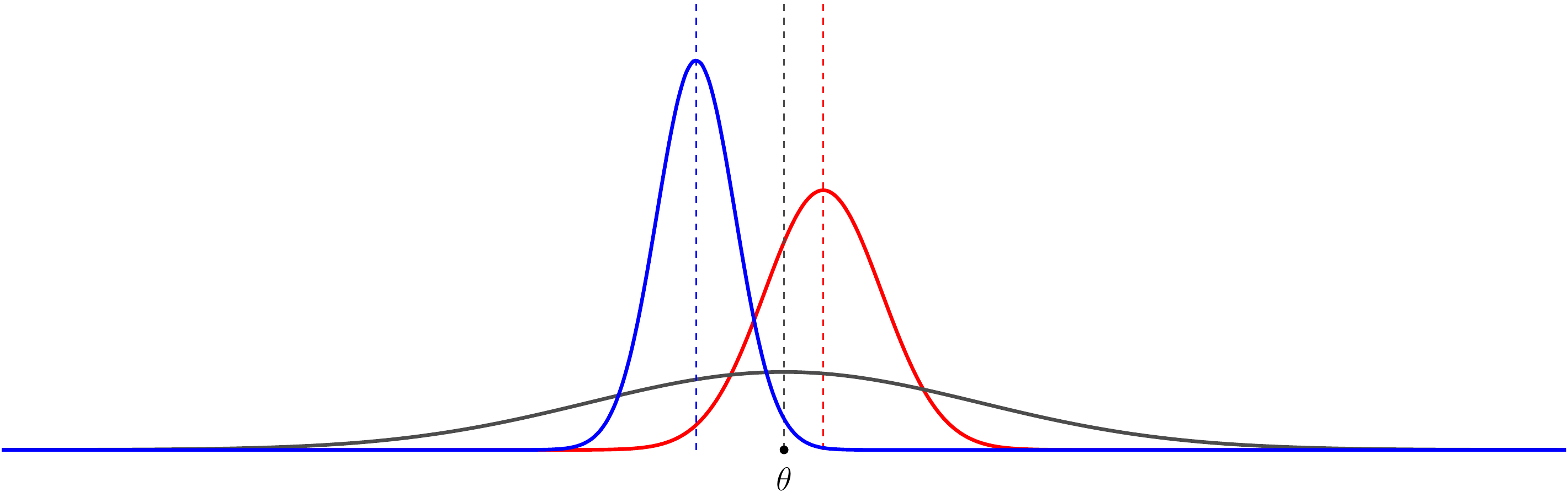
Figure 32.1 shows the distributions of three hypothetical estimators. Although the gray estimator is unbiased, the red estimator tends to be “closer” to the true \(\theta\). It is biased, but the reduction in variance appears to be worth the small increase in bias. However, we do not always prefer the estimator with lower variance. The blue estimator has an even lower variance, but its bias is so large that it appears to be worse than the gray estimator.
Figure 32.1: Illustration of three estimators of \(\theta\): one unbiased (gray) and two biased (red, blue).
How do we navigate the delicate tradeoff between bias and variance? The next definition is a natural criterion for comparing two estimators. It quantifies how far an estimator \(\hat\theta\) is from the true parameter \(\theta\) on average.
Definition 32.2 (Mean squared error) The mean squared error (or MSE) of an estimator \(\hat\theta\) for estimating a parameter \(\theta\) is \[
\text{MSE} \overset{\text{def}}{=}\text{E}\!\left[ (\hat{\theta} - \theta)^2 \right].
\tag{32.3}\]
Naturally, we prefer the estimator with the smaller MSE. The next theorem is one of those rare results that are useful for computation and offer insight.
Theorem 32.1 (Bias-variance decomposition) The MSE of an estimator \(\hat\theta\) of \(\theta\) can be decomposed as the sum of its squared bias plus its variance:
Notice that \(A\) is random (because it depends on the random variable \(\hat\theta\)), but \(b\) is a constant. Therefore, by linearity of expectation,
The first two terms are the desired decomposition into squared bias plus variance. We just need to show that the last term, the “cross-term”, is zero. But this follows from linearity of expectation: \[
\text{E}\!\left[ (\hat{\theta} - \text{E}\!\left[ \hat{\theta} \right]) \right] = \text{E}\!\left[ \hat{\theta} \right] - \text{E}\!\left[ \hat{\theta} \right] = 0.
\]
Theorem 32.1 formalizes the intuition that estimators should ideally have low bias and low variance. If either bias or variance is large, then the MSE will be large as well. Theorem 32.1 also shows that if an estimator is unbiased, then the MSE is exactly equal to its variance. Thus, among unbiased estimators, the best one is the one with the smallest variance, which justifies the discussion in Section 32.1.
Armed with Theorem 32.1, we can settle whether \(\hat{N}_{\textrm{MLE}+}\) is better than \(\hat{N}_{\textrm{MLE}}\).
Example 32.3 (Comparing German tank estimators via MSE) Consider the German tank problem, where we observe a simple random sample of serial numbers \(X_1, \dots, X_n\) from \(\{ 1, \dots, N \}\). We have considered three estimators of \(N\):
We know that the last two estimators are unbiased, and we showed in Example 32.1 and Example 32.2 that \(\hat N_{\textrm{MLE}+}\) had the lower variance, so \(\hat N_{\textrm{MLE}+}\) is better than \(\hat N_{\text{MoM}}\).
But is \(\hat N_{\textrm{MLE}+}\) better than \(\hat N_{\textrm{MLE}}\)? To compare an unbiased estimator to a biased one, we calculate their MSEs.
Since \(\hat N_{\textrm{MLE}+}\) is unbiased, its MSE is simply its variance: \[
\text{E}\!\left[ (\hat N_{\textrm{MLE}+} - N)^2 \right] = \text{Var}\!\left[ \hat N_{\textrm{MLE}+} \right] = \frac{(N+1)(N-n)}{n(n+2)}.
\tag{32.5}\]
On the other hand, we can use Theorem 32.1 to calculate the MSE of \(\hat{N}_{\textrm{MLE}}\). Notice that we already calculated the bias in Example 31.1 and the variance in Example 32.1. \[
\begin{align}
\text{E}\!\left[ (\hat N_{\textrm{MLE}} - N)^2 \right] &= \text{Var}\!\left[ \hat N_{\textrm{MLE}} \right] + (\text{E}\!\left[ \hat N_{\textrm{MLE}} \right] - N)^2 \\
&= \frac{n(N+1)(N-n)}{(n+1)^2(n+2)} + \left(-\frac{N-n}{n+1}\right)^2 \\
&= \frac{N-n}{n+2} \frac{ n(N+1) + (n+2)(N-n)}{(n+1)^2}.
\end{align}
\tag{32.6}\]
Comparing Equation 32.5 and Equation 32.6, we see that \(\hat{N}_{\textrm{MLE}+}\) has a lower MSE when \[
\frac{N+1}{n} < \frac{ n(N+1) + (n+2)(N-n)}{(n+1)^2}.
\]
When \(n > 1\), this expression simplifies to \[
N > n + 2 + \frac{3}{n-1}.
\] (There is no solution when \(n = 1\), which means that \(\hat N_\textrm{MLE}\) is better when there is only one tank in the sample!)
For \(n > 4\), \(\frac{3}{n-1} < 1\), so this inequality is equivalent to \(N > n+2\) (since \(N\) must be an integer). That is, unless the sample size \(n\) represents (almost) the entire population, \(\hat{N}_{\textrm{MLE}+}\) will have smaller MSE than \(\hat{N}_{\textrm{MLE}}\). This makes intuitive sense: if \(n\) is very close to \(N\), then it is highly likely that the maximum serial number in the sample is \(N\), in which case the \(\hat{N}_{\textrm{MLE}}\) is exact, while \(\hat{N}_{\textrm{MLE}+}\) overestimates.
Example 32.3 shows that the unbiased estimator does not always outperform the biased one. We can often achieve a significant reduction in variance by introducing a little bias. The delicate balance between the two is called the bias-variance tradeoff.
The next example reinforces the point that a biased estimator can have a lower MSE than an unbiased one.
Example 32.4 (A biased estimator with smaller MSE) Suppose we observe i.i.d. data \(X_1, \dots, X_n\) from an \(\text{Exponential}(\lambda)\) distribution (Definition 22.2), and we want to estimate the mean \(\mu \overset{\text{def}}{=}\text{E}\!\left[ X_1 \right] = 1/\lambda\) of this distribution.
By Proposition 31.1, \(\bar X\) is an unbiased estimator for \(\mu\). (In Exercise 30.8, you showed that it is also the MLE.) Its MSE is therefore given by its variance. We can use Equation 32.2 to compute \(\text{Var}\!\left[ \bar X \right]\). Because the observations are i.i.d., \(\text{Cov}\!\left[ X_i, X_j \right] = 0\). \[
\begin{align}
\text{E}\!\left[ (\bar X - \mu)^2 \right] = \text{Var}\!\left[ \bar{X} \right] &= \frac{1}{n^2} \sum_{i=1}^n \text{Var}\!\left[ X_i \right] \\
&= \frac{1}{n^2} n \frac{1}{\lambda^2} \\
&= \frac{\mu^2}{n}.
\end{align}
\tag{32.7}\]
On the other hand, consider the biased estimator \[
\hat{\mu}_{\text{biased}} = \frac{n}{n+1} \bar X.
\] To compute its MSE, we need to compute its bias \[
\begin{align*}
\text{E}\!\left[ \hat{\mu}_{\text{biased}} \right] - \mu &= \text{E}\!\left[ \frac{n}{n+1} \bar X \right] - \mu & \text{(definition of $\hat\mu_{\text{biased}}$)} \\
&= \frac{n}{n+1} \text{E}\!\left[ \bar X \right] - \mu & \text{(properties of expectation)}\\
&= \frac{n}{n+1} \mu - \mu & \text{($\bar X$ is unbiased)} \\
&= -\frac{\mu}{n+1} & \text{(simplify)}
\end{align*}
\] and variance \[
\text{Var}\!\left[ \hat{\mu}_{\text{biased}} \right] = \text{Var}\!\left[ \frac{n}{n+1} \bar X \right] = \left(\frac{n}{n+1}\right)^2 \text{Var}\!\left[ \bar X \right] = \frac{n}{(n+1)^2}\mu^2
\]
Theorem 32.1 tells us that the MSE of \(\hat{\mu}_{\text{biased}}\) is the squared bias plus the variance: \[
\begin{align}
\text{E}\!\left[ \big(\hat{\mu}_{\text{biased}} - \mu\big)^2 \right] &= \left(-\frac{\mu}{n+1} \right)^2 + \frac{n}{(n+1)^2}\mu^2 \\
&= \frac{\mu^2}{n+1}.
\end{align}
\tag{32.8}\]
In Equation 32.7, we computed the variance of the sample mean of i.i.d. exponential random variables. We summarize the general result for any i.i.d. random variables.
Proposition 32.1 (Variance of the sample mean of i.i.d. random variables) Let \(X_1, \dots, X_n\) be i.i.d. random variables from any distribution with finite variance \(\sigma^2 = \text{Var}\!\left[ X_1 \right]\). Then the variance of the sample mean (Equation 31.5) is \[
\text{Var}\!\left[ \bar{X} \right] = \frac{\sigma^2}{n}.
\tag{32.9}\]
Proof
We use Equation 32.2 to compute \(\text{Var}\!\left[ \bar X \right]\). Because the observations are i.i.d., \(\text{Cov}\!\left[ X_i, X_j \right] = 0\). \[
\begin{align}
\text{Var}\!\left[ \bar{X} \right] &= \frac{1}{n^2} \sum_{i=1}^n \text{Var}\!\left[ X_i \right] \\
&= \frac{1}{n^2} n \sigma^2 \\
&= \frac{\sigma^2}{n}.
\end{align}
\]
Notice that Proposition 32.1 is more restrictive than Proposition 31.1, where we showed that \(\text{E}\!\left[ \bar X \right] = \mu\) for any identically distributed random variables, even if they are not independent. By contrast, Proposition 32.1 only holds if the random variables are also independent; otherwise, we need to use the more general formula Equation 32.2.
Because \(\bar X\) is unbiased for \(\mu\), its MSE is the variance, so Equation 32.9 is also the MSE of the sample mean for estimating \(\mu\).
32.3 Estimating the Variance
We saw in Proposition 31.1 that if we observe i.i.d. random variables \(X_1, \dots, X_n\) from any distribution, then a general estimator for the mean \(\mu = \text{E}\!\left[ X_1 \right]\) is the sample mean. Is there a similar estimator for the variance \(\sigma^2 = \text{Var}\!\left[ X_1 \right]\)?
Since \(\text{Var}\!\left[ X_1 \right] \overset{\text{def}}{=}\text{E}\!\left[ (X_1 - \mu)^2 \right]\), one idea is to replace all of the expectations by sample averages. That is, we plug in \(\bar X\) for \(\mu\) and estimate the variance as \[
\hat\sigma^2 = \frac{1}{n} \sum_{i=1}^n (X_i - \bar X)^2.
\tag{32.10}\] Is this a good estimator? The following lemma, which is really just a discrete version of the bias-variance decomposition (Theorem 32.1), will help us answer this question. The result is not hard to prove by direct algebra, but Exercise 32.9 suggests a slicker way.
Lemma 32.1 (Sum-of-squares decomposition) Let \(a_1, \dots, a_n\) be any real numbers, and define \(\bar a \overset{\text{def}}{=}\frac{1}{n}\sum_{i=1}^n a_i\). Then, for any real number \(c\),
Example 32.5 (Bias of the variance estimator \(\hat\sigma^2\)) Applying Lemma 32.1 to the random variables \(X_1, X_2, \dots, X_n\), \[
\frac{1}{n} \sum_{i=1}^n (X_i - \mu)^2 = \underbrace{\frac{1}{n} \sum_{i=1}^n (X_i - \bar X)^2}_{\hat\sigma^2} + (\bar X - \mu)^2.
\] The first term on the right-hand side is the variance estimator \(\hat\sigma^2\). So we can express the estimator alternatively as \[ \hat\sigma^2 = \frac{1}{n} \sum_{i=1}^n (X_i - \mu)^2 - (\bar X - \mu)^2. \tag{32.12}\] In this form, we can calculate the bias. \[\begin{align}
\text{E}\!\left[ \hat\sigma^2 \right] &= \text{E}\!\left[ \frac{1}{n} \sum_{i=1}^n (X_i - \mu)^2 \right] - \text{E}\!\left[ (\bar X - \mu)^2 \right] \\
&= \text{E}\!\left[ (X_i - \mu)^2 \right] - \text{E}\!\left[ (\bar X - \mu)^2 \right] \\
&= \text{Var}\!\left[ X_i \right] - \text{Var}\!\left[ \bar X \right] \\
&= \sigma^2 - \frac{\sigma^2}{n} \\
&= \frac{n-1}{n} \sigma^2,
\end{align}\] so its bias is \[
\text{E}\!\left[ \hat\sigma^2 \right] - \sigma^2 = \left(\frac{n-1}{n} \sigma^2 - 1\right)\sigma^2 = -\frac{\sigma^2}{n}.
\]
But Example 32.5 immediately suggests an unbiased estimator of \(\sigma^2\): we can simply scale \(\hat\sigma^2\) by \(\frac{n}{n-1}\).
Proposition 32.2 (A general unbiased estimator for the variance) Let \(X_1, \dots, X_n\) be i.i.d. random variables from any distribution with finite variance \(\sigma^2 \overset{\text{def}}{=}\text{Var}\!\left[ X_1 \right]\).
Then, the sample variance\[
S^2 \overset{\text{def}}{=}\frac{n}{n-1} \hat\sigma^2 = \frac{1}{n-1} \sum_{i=1}^n (X_i - \bar X)^2
\tag{32.13}\] is an unbiased estimator of \(\sigma^2\).
Since \(S^2\) is unbiased for \(\sigma^2\), its MSE is just its variance.
32.4 Exercises
Exercise 32.1 (Evaluating the Poisson MLE) Let \(X_1, \dots, X_n\) be i.i.d. \(\text{Poisson}(\mu)\). In Exercise 31.1, you calculated the bias of the MLE.
What is the MSE of the MLE?
How does the MSE change as you collect more data (i.e., as \(n\) increases)?
Exercise 32.2 (Another unbiased estimator of the Poisson mean) Recall Exercise 30.2, where you calculated the MLE of \(\mu\) for the V-1 flying bombs data.
Propose another estimator (besides the MLE) that uses all of the data and is unbiased for \(\mu\). (Hint: What is \(\text{Var}\!\left[ X_1 \right]\)?)
Calculate this estimate on the V-1 flying bombs data and compare it with the maximum likelihood estimate.
Which estimate would you trust more? Write a simulation to investigate.
Exercise 32.3 (Evaluating the normal variance MLE when mean is known) Let \(X_1, \dots, X_n\) be i.i.d. \(\text{Normal}(\mu, \sigma^2)\), where \(\mu\) is known (but \(\sigma^2\) is not). In Exercise 31.5, you found the MLE of \(\sigma^2\). What is the MSE of this estimator?
Exercise 32.4 (Comparing estimators for the uniform distribution) Recall \(\hat{\theta}_{\textrm{MLE}}\) and \(\hat{\theta}_{\textrm{MLE}+}\) from Exercise 31.6. Which is the better estimator of \(\theta\)?
Exercise 32.5 (Minimizing the MSE of an exponential estimator) Let \(X_1, \dots, X_n\) be i.i.d. \(\text{Exponential}(\lambda)\). Consider estimators of the form \[
\hat{\mu}_\alpha = \alpha \bar{X},
\] for \(\mu = 1/\lambda\). For example \(\hat\mu_1\) is the MLE and \(\hat\mu_{\frac{n}{n+1}}\) is the estimator in Example 32.4.
For which value of \(\alpha\) is the MSE of \(\hat{\mu}_\alpha\) minimized?
Exercise 32.6 (Minimizing the MSE of a uniform estimator) Let \(X_1, \dots, X_n\) be i.i.d. \(\text{Uniform}(0,\theta)\). Consider \[
\hat{\theta}_\alpha = \alpha \bar{X},
\] an estimator of \(\theta\). For which value of \(\alpha\) is the MSE of \(\hat{\theta}_\alpha\) minimized?
Exercise 32.7 (Combining two estimators) Suppose we have two independent estimators \(\hat{\theta}_1\) and \(\hat{\theta}_2\), both of which are unbiased for a parameter \(\theta\). Can we combine these two estimators to create an even better estimator?
Consider linear combinations of the two estimators \[
\hat{\theta}_{\text{combined}} = w_1 \hat{\theta}_1 + w_2 \hat{\theta}_2.
\] What must be true of \(w_1\) and \(w_2\) in order for \(\hat{\theta}_{\text{combined}}\) to be unbiased?
What choice of \(w_1\) and \(w_2\) leads to the “best” unbiased estimator? (Your answer should depend on \(\text{Var}\!\left[ \hat\theta_1 \right]\) and \(\text{Var}\!\left[ \hat\theta_2 \right]\).)
Exercise 32.8 (Random sample with replacement) Let \(c_1, c_2, \dots, c_N\) be a population of \(N\) values, and let \(X_1, X_2, \dots, X_n\) be a random sample of size \(n\) drawn from this population with replacement (so that the same \(c_i\) can be selected multiple times).
Show that \(\bar X\) is an unbiased estimator of the population mean \[\bar c \overset{\text{def}}{=}\frac{1}{N} \sum_{i=1}^N c_i.\]
Calculate \(\text{Var}\!\left[ \bar X \right]\) and the MSE of \(\bar X\) for estimating the population mean \(\bar c\).
Exercise 32.9 (Proof of the sum-of-squares decomposition) Prove Lemma 32.1.
Hint: Define \(\hat\theta\) to be a random variable that takes on the values \(\{ a_1, \dots, a_n \}\), each with probability \(1/n\), and apply Theorem 32.1.
Exercise 32.10 (Comparing variance estimators) Consider the two estimators of \(\sigma^2\) in Section 32.3. Express the MSE of \(\hat\sigma^2\) in terms of the MSE of \(S^2\). Is one necessarily better than the other?
Exercise 32.11 (Linear unbiased estimators of the mean) Let \(X_1, \dots, X_n\) be i.i.d. random variables with \(\text{E}\!\left[ X_i \right] = \mu\).
What condition on the constants \(w_1, \dots, w_n\) is necessary for \(\hat\mu = w_1 X_1 + \dots + w_n X_n\) unbiased for \(\mu\)?
What value of \(w_1, \dots, w_n\) ensures that \(\hat\mu\) is unbiased and minimizes \(\text{Var}\!\left[ \hat\mu \right]\)?