20 Transformations
$$
$$
\[ \def\mean{\textcolor{red}{1.2}} \]
In many applications, we care not just about a random variable \(X\), but about some transformation of it, \(Y = g(X)\). This transformation produces a new random variable \(Y\) with its own distribution.
One situation in which transformations naturally arise is unit conversion. For example:
- We modeled Jackie Joyner-Kersee’s long jump distance \(X\) in meters, but the long jump distance is often reported in centimeters. The distance in centimeters is a random variable \(Y = 100X\).
- If the daily high temperature in London (measured in Celsius) is a random variable \(C\), then an American tourist might want to know the temperature in Fahrenheit, which is a random variable \(F = \frac{9}{5}C + 32\).
In this chapter, we will learn how to derive the PDF of \(Y = g(X)\) from the PDF of \(X\).
20.1 The PDF of a Transformed Random Variable
Suppose we construct a “random” square as follows. First, we pick a side length \(X\) which is “equally likely” to be any number between \(0\) and \(1\). That is, the PDF of \(X\) is \[ f_X(x) = \begin{cases} 1 & 0 < x < 1 \\ 0 & \text{otherwise} \end{cases}. \] Then, we draw a square with sides of length \(X\). The area of the square is \[ Y = X^2. \] Notice that \(Y\) is a transformation of \(X\). What is the PDF of \(Y\)?
If we square a number between \(0\) and \(1\), the result is also a number between \(0\) and \(1\). But is \(Y\) also “equally likely” to be any number between \(0\) and \(1\)? We can find out with a simulation.
Clearly, the probability is more concentrated near \(0\), so the PDF of \(Y\) is not the same as the PDF of \(X\). In hindsight, this is not surprising: when a number between \(0\) and \(1\) is squared, the result is smaller. So if the original numbers were equally likely to be between \(0\) and \(1\), the squared numbers should be more likely to be near \(0\).
Here is another way to explain the observation above: the probability that \(X\) is below \(0.5\) is 50%. But values of \(X\) below \(0.5\) correspond to values of \(Y\) below \((0.5)^2 = 0.25\). That is, although \(Y\) can be any number between \(0\) and \(1\), 50% of the probability is below \(0.25\).
Now, we develop a strategy for deriving the PDF of \(Y\), which is based on what we learned in Chapter 18.
Let’s apply this strategy to the example above.
In general, we apply the strategy in this section to determine the PDF of a transformed random variable \(Y = g(X)\). However, for specific classes of transformations \(g\), there are simple formulas for the PDF. The next two sections explore two important classes of transformations.
20.2 Location-Scale Transformations
In this section, we will explore an important class of transformations called location-scale transformations.
Let’s examine location transformations first. If we add \(b\) to a random variable \(X\), then the support and all the probabilities should shift by \(b\). This is illustrated in Figure 20.1.
Now let’s develop this observation into a formula.
Next, let’s examine scale transformations. Suppose we multiply a random variable \(X\) by the constant \(a = 1.5\), producing a new random variable \(Y = 1.5 X\). The support will be stretched out by a factor of \(1.5\) so that if the possible values of \(X\) range from \(0\) to \(6\), the possible values of \(Y\) will range from \(0\) to \(9\). Furthermore, the PDF is “squashed” by a factor of \(1.5\). This effect is illustrated in Figure 20.2.
While it should be clear that a scale transformation stretches the PDF, it may be less obvious why it also squashes the PDF. Here are two ways to see that the squashing is necessary:
- If we stretched the PDF without squashing it, there would be too much area under the PDF. The total area under a PDF must equal 1, before and after the transformation.
- Think of a scale transformation as a change of units, and consider the units on the vertical axis. If \(X\) is in meters and \(Y = 100 X\) is in centimeters, then the units on the vertical axis change from “probability per meter” to “probability per centimeter”. One centimeter is shorter than one meter, so there should be less probability per centimeter than per meter!
Now that we understand the intuition, we can formalize the result.
Finally, a location-scale transformation is just a scale transformation followed by a location transformation. So we can obtain the next result by simply combining Proposition 20.1 and Proposition 20.2.
Now let’s apply location-scale transformations to an example.
Example 20.2 (Converting Celsius to Fahrenheit) In Example 18.5, we modeled the daily high temperature \(C\) as a continuous random variable with PDF \[ f_C(x) = \frac{1}{k} e^{-x^2/18}; -\infty < x < \infty, \] where \(k\) was a constant that makes the total area equal to 1. We determined the constant \(k\) to be about \(7.5\). This PDF was graphed in Figure 18.7.
An American visitor to Iqaluit might want to know the temperature in Fahrenheit. But this is just a location-scale transformation of the temperature in Celsius! In particular: \[ F = g(C) = \textcolor{green}{\frac{9}{5}} C + \textcolor{orange}{32}. \]
We can derive the PDF of \(F\) using Proposition 20.3 above, with \(a = \textcolor{green}{9/5}\) and \(b = \textcolor{orange}{32}\). Therefore, the PDF of \(F\) is:
\[ \begin{aligned} f_F(x) &= \frac{1}{\textcolor{green}{9/5}} f_C\left(\frac{x-\textcolor{orange}{32}}{\textcolor{green}{9/5}}\right) \\ &= \frac{1}{\textcolor{green}{9/5}} \frac{1}{k} e^{\displaystyle -\left( \frac{x-\textcolor{orange}{32}}{\textcolor{green}{9/5}} \right)^2 / 18} \\ &\approx \frac{1}{13.53579} e^{-(x - 32)^2 / 58.32} \end{aligned} \tag{20.4}\]
Let’s graph the PDF in Fahrenheit (Equation 20.4):
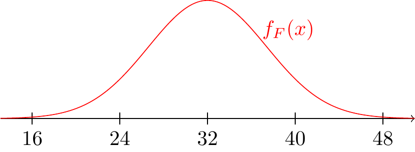
Compared to Figure 18.7, this PDF is centered around the freezing point in Fahrenheit (\(32^\circ\)) instead of the freezing point in Celsius (\(0^\circ\)).
20.3 The Probability Integral Transform
Let \(X\) be a continuous random variable with CDF \(F(x)\). Then \(U = F(X)\) is also a continuous random variable. What is the distribution of \(U\)?
This particular class of transformations, where we plug a random variable into its own CDF, is called the probability integral transform. At first, it may not be clear why anyone would do such a thing, but we will see that it is actually one of the most useful tricks in all of probability.
What use is knowing that \(U = F(X)\) has a standard uniform distribution? Some direct applications of the probability integral transform are suggested in Exercise 20.6. But the most compelling application derives from the inverse transformation: \(X = F^{-1}(U)\). This suggests that we can simulate values of \(X\) from any (continuous) distribution by first simulating \(U\) and then calculating \(F^{-1}(U)\). This trick is called inverse transform sampling, and it follows immediately from Theorem 20.1.
Proposition 20.4 is useful because a programming language may not have a built-in function to simulate from the distribution you want, but every programming language has a function to generate uniform random numbers between 0 and 1.
20.4 Exercises
Exercise 20.1 (Proving Proposition 20.2) Complete the proof of Proposition 20.2 by showing that Equation 20.2 also holds when \(a < 0\).
Hint: Remember that when you multiply or divide both sides of an inequality by a negative number, the direction of the inequality flips!
Exercise 20.2 (Heptathlon score) The long jump is one of the seven contests in the heptathlon. Competitors earn points for each event in the heptathlon, and the competitor with the most total points is the winner. But the heptathlon consists of many different contests:
- The long jump and high jump are measured in distance.
- The shotput and javelin are also measured in distance, but the distances are much longer.
- The 200m, 800m, and 100m hurdles are measured in time.
How do we put all these different contests on the same scale? The result of each heptathlon contest is transformed in a different way so that the resulting points are on a similar scale. For example, the transformation that is used for scoring the long jump in the women’s heptathlon is: \[ g(x) = 124.7435 (x - 2.1)^{1.41}; x \geq 2.1, \] where \(x\) is the distance in meters. Joyner-Kersee was also a gold-medal heptathlete. If we want to know how many points she earns in the heptathlon from the long jump, then we need to study the random variable \(S = g(X)\).
Let’s assume that Jackie Joyner-Kersee’s long jump \(X\) is equally likely to be any distance between 6.3 and 7.5 meters, as in Example 18.3. Determine the PDF of \(S\), the contribution to her score from the long jump.
Exercise 20.3 (Reaction rates) In a chemistry lab, students are running a reaction under what they think are identical conditions. However, in reality, each beaker sits in slightly different ambient temperature. Let \(T\) be the temperature, in Kelvin, of a randomly chosen beaker. Assume \(T\) is equally likely to be between 293 and 295 Kelvins.
Reaction rate constant \(K\), which measures the frequency of collisions resulting in a reaction, can be modeled by \[ K = A e^{-\frac{E_a}{RT}}, \] where \(A\) is the pre-exponential factor constant, \(E_a\) is the activation energy of the reaction, \(R\) is the gas constant, and \(T\) is the temperature. Note that \(A\), \(E_a\), and \(R\) are all positive constants.
- What is the range of possible values of \(K\)?
- Derive the PDF of \(K\).
- Compute \(\text{E}\!\left[ K \right]\).
Exercise 20.4 (Simulating a half-triangle) Write code to simulate a random variable \(X\) with the half-triangle PDF \[ \begin{equation} f(x) = \begin{cases} 1 - \frac{x}{2} & 0 \leq x < 2 \\ 0 & \text{otherwise} \end{cases}, \end{equation} \tag{20.5}\] using inverse transform sampling from Proposition 20.4.
Exercise 20.5 (Power dissipation) A bin is labeled “\(10\Omega\) resistors.” Due to manufacturing variation, the true resistance \(R\) of a randomly selected resistor from the bin is equally likely to be between \(9\) and \(11\) ohms.
In the circuit these resistors will be used in, each resistor is placed across a voltage source of \(V = 110\) volts. The power \(W\) dissipated as heat follows the equation \[ W = \frac{V^2}{R}. \] We care about \(W\) since it will tell use whether the resistor is running too hot.
- Find the PDF of \(W\). Note that \(W\) is a decreasing function of \(R\).
- Compute \(P(W > 1200)\), the probability that a randomly chosen resistor will overheat at this voltage.
Exercise 20.6 (Distribution of \(p\)-value) A common problem in statistics is to determine whether data \(x\) is too large to have plausibly come from a distribution with CDF \(F\). One way to do this is to calculate the probability of observing \(x\) or greater, \(p = 1 - F(x)\), and if this \(p\)-value is small (say, less than \(.05\)), then we conclude that \(x\) did not come from that distribution.
Now, suppose that the data \(X\) is a random variable that really does have CDF \(F\). What is the distribution of the \(p\)-value?