23 Joint Distributions
$$
$$
\[ \def\y{\textcolor{red}{y}} \]
In this chapter, we describe the distributions of multiple continuous random variables. To get the most out of this chapter, please reread Chapter 13 to review how we described the distributions of multiple discrete random variables. You will see that many concepts are identical, except with PMFs replaced by PDFs and sums replaced by integrals.
23.1 Joint PDF
In Chapter 13, we described the distribution of two discrete random variables \(X\) and \(Y\) by their joint PMF \[ f_{X,Y}(x,y) = P(X = x, Y = y). \] The joint PMF is useless for continuous random variables \(X\) and \(Y\) because \[ P(X = x, Y = y) = 0 \] for any values \(x\) and \(y\). Instead, we shall describe the distribution of two continuous random variables by their joint PDF.
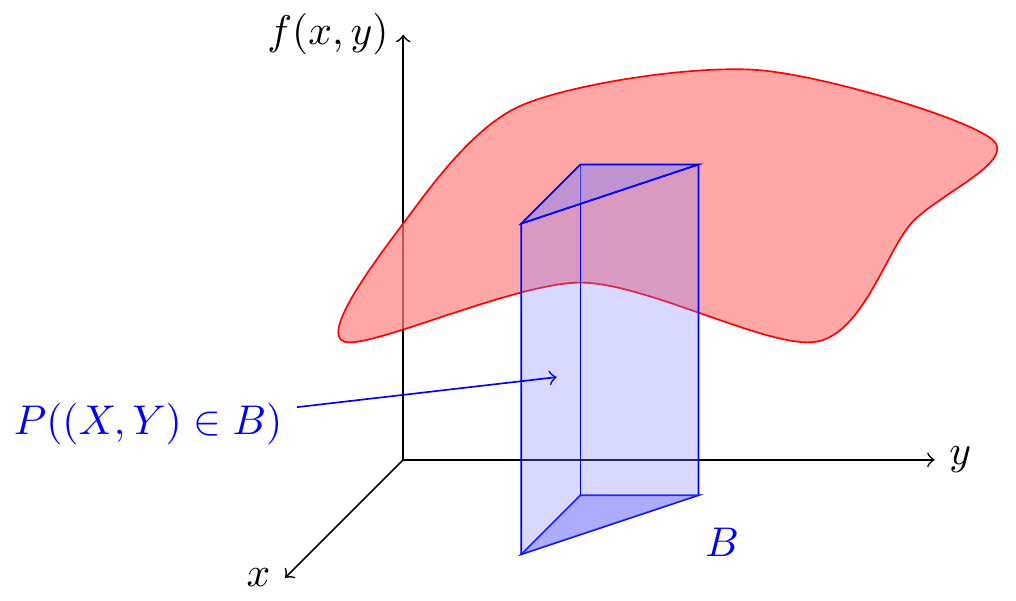
The joint PDF is the natural extension of the PDF (Chapter 18) to multiple random variables. Whereas a PDF \(f_X(x)\) could be visualized as a curve; the joint PDF \(f_{X, Y}(x, y)\) is a surface over the \(xy\)-plane, as shown in Figure 23.1.
The probability of any event \(B\) is the volume under this surface. We begin with an example where it is easy to determine this volume geometrically.
Example 23.1 (When Harry met Sally?) Harry and Sally plan to meet at Katz’s Deli for lunch. Let \(X\) and \(Y\) be the times that Harry and Sally arrive, respectively, in minutes after noon.
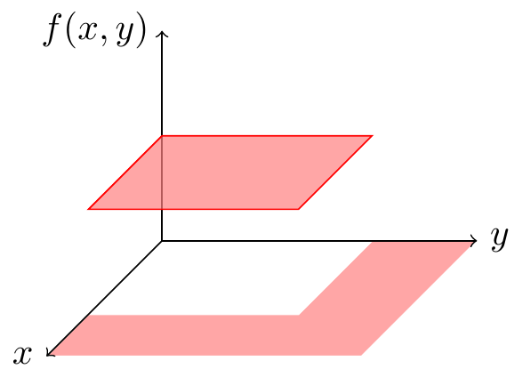
Suppose the joint PDF of \(X\) and \(Y\) is \[ f_{X,Y}(x,y) = \begin{cases} c, & 0 \leq x \leq 30, 0 \leq y \leq 60 \\ 0, & \text{else} \end{cases}, \] where \(c\) is a constant. That is, the surface is flat over the support of the distribution, as shown in Figure 23.2.
In order to calculate any probabilities, we first need to determine the height of this surface. To do so, we use the fact that the total probability must be \(1\); that is, the total volume under the surface must be \(1\). Since the volume under the surface is a rectangular prism, its volume is \[ \begin{align} \text{total volume under surface} &= \text{base} \cdot \text{height} \\ &= (30 \cdot 60) \cdot c. \end{align} \] Setting this total volume equal to \(1\), we obtain \[ c = \frac{1}{1800}. \]
Using this information, we can calculate probabilities. For example, suppose Harry and Sally will each wait \(15\) minutes for the other to arrive. What is the probability that they meet? In other words, we want to determine \[ P((X, Y) \in B) = P(|X - Y| < 15). \]
To do this, we determine the set \(B\) in the \(xy\)-plane, and calculate the volume under the joint PDF above \(B\), the blue prism shown in Figure 23.3.
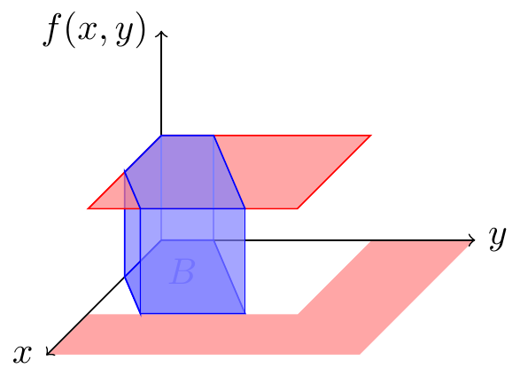
Figure 23.3 shows the full picture, but it is unwieldy to draw. For calculating probabilities, we usually just need a bird’s-eye view of the event \(B\). Consider Figure 23.3 from the perspective of Rand the Raven, who is flying high above the \(xy\)-plane. The picture from Rand’s perspective is shown in Figure 23.4.
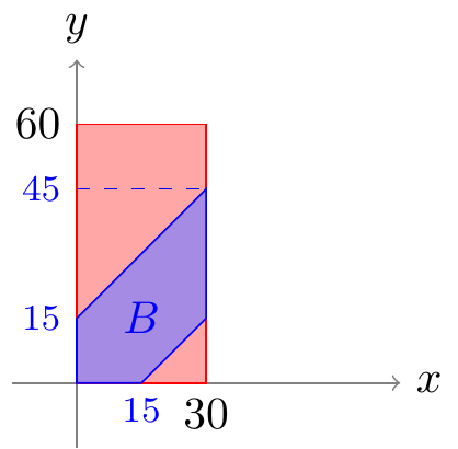
To calculate the volume of the prism, we just need to determine the area of its base \(B\) in Figure 23.4 and multiply by the height of the surface, \(c = \frac{1}{1800}\). That is, \[ \begin{align} P(|X - Y| < 15) &= \text{volume under surface above $B$} \\ &= (\text{area of $B$}) \cdot \text{height of surface} \end{align} \]
The area of \(B\) can be determined using basic geometry. One way is to take the area of the \(30 \times 45\) rectangle and subtract the areas of the two triangles. \[ \begin{align} (\text{area of $B$}) &= 30 \cdot 45 - \frac{1}{2} \cdot 30 \cdot 30 - \frac{1}{2} \cdot 15 \cdot 15 \\ &= 787.5 \end{align} \]
Therefore, the probability that Harry and Sally meet is \[ P(\lvert X - Y \rvert < 15) = 787.5 \cdot \frac{1}{1800} = .4375. \]
We were able to solve Example 23.1 using geometry because the joint PDF surface, \(f_{X, Y}(x, y)\), was flat. However, in general, the joint PDF surface will be curved, and integration is necessary to calculate volumes under the surface. Specifically, we will need to calculate the double integral of the joint PDF over \(B\):
\[ P((X, Y) \in B) = \iint_B f_{X, Y}(x, y)\,dx\,dy. \]
The next example illustrates how integration can be used to calculate a probability involving two random variables.
Example 23.2 (Blood Types) The ABO blood group system is used to classify human blood types. These blood types are caused by three genetic variants, or alleles, on chromosome 9: O, A, and B. The frequencies of these three alleles vary from population to population. In one population, it might be 70% O, 15% A, and 15% B, while in another population, it might be 60% O, 10% A, and 30% B.
The frequencies of these three alleles in a population are random variables; let’s call them \(X\), \(Y\), and \(Z\), respectively. The joint distribution of \(X\) and \(Y\) can be modeled by \[ f(x, y) = \begin{cases} 12 x^2 & x, y > 0, x + y < 1 \\ 0 & \text{otherwise} \end{cases}. \] Note that \(X + Y + Z = 1\), so \(Z\) is determined once we know \(X\) and \(Y\).
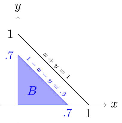
What is \(P(Z > .3) = P(1 - X - Y > .3)\), the probability that more than 30% of the alleles in a population will be B? To calculate this probability, we sketch a bird’s-eye view of the support of the distribution and the set \(B = \{ 1 - X - Y > .3 \}\) in Figure 23.5.
The surface \(f(x, y)\) is not flat, so to calculate the volume under the surface, we will need to calculate a double integral over \(B\). To evaluate this integral, we convert the double integral into an iterated integral.
\[ \begin{aligned} P(1 - X - Y > .3) &= \iint_B f(x, y)\,dx\,dy \\ &= \int_{\textcolor{red}{0}}^{\textcolor{red}{.7}} \underbrace{\int_0^{.7 - \y} 12 x^2 \,dx}_{4x^3 \Big|_0^{.7 - \y}} \,d\y \\ &= \int_{\textcolor{red}{0}}^{\textcolor{red}{.7}} 4 (.7 - \y)^3 \,d\y \\ &= .2401. \end{aligned} \]
We would have arrived at the same answer if we had set up the iterated integral in the other order, \(dy\,dx\) instead of \(dx\,dy\).
\[ \begin{aligned} P(1 - X - Y > .3) &= \int_{0}^{.7} \int_0^{.7 - x} 12 x^2 \,dy\,dx \\ &= \int_{0}^{.7} 12 x^2 \int_0^{.7 - x} 1 \,dy\,dx \\ &= \int_{0}^{.7} 12 x^2 (.7 - x) \,dx \\ &= .2401. \end{aligned} \]
So there is only about a \(.24\) probability that the frequency of B alleles in a population exceeds 30%.
23.2 Marginal Distribution
In Section 13.2, we saw that we can recover the PMF of a discrete random variable \(X\) from the joint PMF of \(X\) and \(Y\), by summing over all the possible values of \(Y\): \[ f_X(x) = \sum_y f_{X, Y}(x, y). \]
For continuous random variables, the idea is the same, except we integrate the PDF instead of summing the PMF.
Let us revisit Example 23.1 and determine the marginal distributions of the times that Harry and Sally arrive.
In Example 23.3, the joint PDF ends up being the product of the marginal PDFs: \[ f_{X,Y}(x,y) = \frac{1}{1800} = \frac{1}{30} \cdot \frac{1}{60} = f_X(x) f_Y(y) \] for \(30 < x < 60, 0 < y < 60\).
This proves to be a useful characterization of independence for continuous random variables.
The next example illustrates the importance of respecting the support of the distribution when calculating marginal PDFs.
Example 23.4 (Marginal distribution of allele frequencies) In Example 23.2, we examined a particular model for the joint distribution of the allele frequencies of the O and A blood types.
The marginal distribution of \(X\), the allele frequency of the O blood type, is \[ f_X(x) = \int_{-\infty}^\infty f_{X, Y}(x, y)\,dy. \]
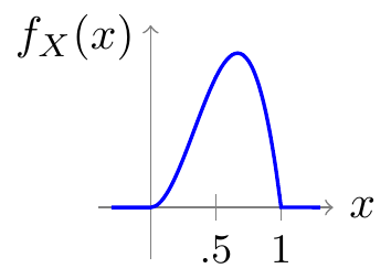
However, the support of this joint distribution is \[ \{ (x, y): x, y > 0, x + y < 1 \}. \] This support was illustrated in Figure 23.5. For a given value of \(x\), the values of \(y\) that are in the support are \((0, 1 - x)\). Therefore: \[ f_X(x) = \int_0^{1 - x} 12x^2\,dy = 12 x^2 (1 - x) \qquad 0 < x < 1. \tag{23.2}\]
Equation 23.2 is graphed in Figure 23.6. Populations are more likely than not to have more than 50% O alleles.
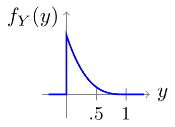
Similarly, the marginal PDF of \(Y\), the frequency of the A allele, is \[ f_Y(y) = \int_0^{1 - y} 12x^2\,dx = 4(1 - y)^3 \qquad 0 < y < 1. \tag{23.3}\]
Equation 23.3 is graphed in Figure 23.7. Populations are most likely to have a small frequency of A alleles.
Notice that the product of the marginal PDFs is \[f_X(x) f_Y(y) = 48 x^2 (1 - x)(1 - y)^3\] for \(0 < x, y < 1\), which is very different from the joint PDF \(f_{X, Y}(x, y)\). Therefore, \(X\) and \(Y\) are not independent. This is intuitive because the frequencies of the alleles must add up to 1, so an increase in the frequency of one allele must be associated with a decrease in another.
23.3 Conditional Distribution
The conditional PDF is a way to describe information that one random variable provides about another. The definition of conditional PDF is the continuous analog of Definition 13.4.
23.4 Further Examples
Example 23.7 (Queueing theory) You and a friend go to an amusement park. There are lines at the gate to enter the park. To enter the park as quickly as possible, you and your friend split up and each get into a different line. You get into a line whose waiting time is \(X\), while your friend gets into a line whose waiting time is \(Y\).
Problems like this are the subject of queueing theory, a branch of applied mathematics that studies the behavior of queues, or lines. In queueing theory, it is common to model the waiting times as exponential random variables.
Suppose \(X \sim \text{Exponential}(\lambda_1)\) and \(Y \sim \text{Exponential}(\lambda_2)\). Because \(X\) and \(Y\) represent the waiting times of two different lines, it makes sense to assume that they are independent. Then, their joint PDF, by Definition 23.2, is \[ f(x, y) = \lambda_1 e^{-\lambda_1 x} \cdot \lambda_2 e^{-\lambda_2 y} \] for \(x, y > 0\).
What is the probability that you enter the park before your friend, \(P(X < Y)\)? This event is sketched in Figure 23.8.
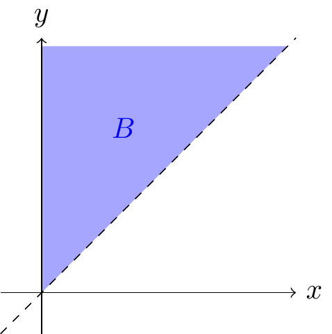
We can calculate this probability by setting up a double integral: \[ \begin{align*} P(X < Y) &= \int_0^\infty \int_x^\infty \lambda_1 e^{-\lambda_1 x} \cdot \lambda_2 e^{-\lambda_2 y} \, dy \, dx \\ &= \int_0^\infty \lambda_1 e^{-\lambda_1 x} \underbrace{\int_x^\infty \lambda_2 e^{-\lambda_2 y} \,dy}_{e^{-\lambda_2 x}} \, dx \\ &= \int_0^\infty \lambda_1 e^{-(\lambda_1 + \lambda_2) x} \, dx \\ &= \frac{\lambda_1}{\lambda_1 + \lambda_2}. \end{align*} \]
To check the plausibility of this answer, suppose that the two lines move at the same rate, \(\lambda_1 = \lambda_2\). By symmetry, since the two lines have identically distributed waiting times, you and your friend should be equally likely to enter first. Therefore, \(P(X < Y) = P(Y < X) = \frac{1}{2}\), which agrees with the formula above.
Now, suppose that you get into a line that moves at a faster rate than your friend, \(\lambda_1 > \lambda_2\). You should be more likely than your friend to get into the park first. This agrees with the formula above, which implies \(P(X < Y) > \frac{1}{2}\).
Example 23.7 illustrates that there is sometimes a way to avoid double integrals in most practical problems. When the distribution is uniform, as in Example 23.1, the probability can be calculated geometrically. When the random variables have the same distribution, we can appeal to symmetry. We will see more techniques in the upcoming chapters.
The next example is a surprising application of joint PDFs. In Section 22.3, we saw that the PDF of the standard normal distribution is \[ f_Z(x) = \frac{1}{\sqrt{2\pi}} e^{-x^2/2}, \qquad -\infty < x < \infty. \] Where does the normalizing constant \(1/\sqrt{2\pi}\) come from? To answer this question, we will first make the problem more complicated by considering the joint distribution of two independent standard normal random variables.
Example 23.9 (Normalizing constant of the standard normal) Determining the normalizing constant \(k\) of the standard normal is not straightforward because there is no “simple” expression for the indefinite integral \(\int e^{-x^2/2}\,dx\). (If you don’t believe it, try to find the antiderivative!)
The solution is to introduce two independent standard normal random variables. Let’s call them \(X\) and \(Y\). Because they are independent, their joint PDF must be the product of the marginal PDFs: \[ f(x, y) = f_X(x) \cdot f_Y(y) = \frac{1}{k} e^{-x^2/2} \cdot \frac{1}{k} e^{-y^2/2} = \frac{1}{k^2} e^{-(x^2 + y^2)/2}. \] As we saw above, the total volume under any joint PDF must equal one.
But this volume can be obtained as a solid of revolution! Specifically, the solid under this curve can be obtained by rotating the red shaded region in Figure 23.9 around the vertical axis.
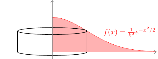
The volume of this solid of revolution is most easily calculated using cylindrical shells. Each shell has a height of \(f(x) = \frac{1}{k^2} e^{-x^2/2}\) and a base with area \(2\pi x\,dx\), so the total volume is \[ \begin{align*} \text{Total Volume} &= \int_0^\infty \frac{1}{k^2} e^{-x^2/2} \cdot 2\pi x\,dx \\ &= \frac{2\pi}{k^2} \int_0^\infty e^{-x^2/2} \cdot x \,dx \\ &= \frac{2\pi}{k^2} \left[ -e^{-x^2/2} \right]_0^\infty \\ &= \frac{2\pi}{k^2}. \end{align*} \] Since we know the total volume must be one, we can solve for \(k\): \[ \begin{align*} \frac{2\pi}{k^2} &= 1 & \Longrightarrow & & k &= \sqrt{2\pi}. \end{align*}\]