In Chapter 23, we learned that the distribution of multiple continuous random variables could be described completely by the joint PDF. However, the joint PDF contains more information than is necessary for most problems. In this chapter, we will summarize random variables by calculating expectations of the form \(\text{E}\!\left[ g(X, Y) \right]\). All of the results in this chapter are analogous to the results in Chapter 14 for discrete random variables, except with PDFs instead of PMFs and integrals instead of sums.
2D LotUS
The general tool for calculating expectations of the form \(\text{E}\!\left[ g(X, Y) \right]\) is 2D LotUS. It is the natural generalization of LotUS from Theorem 21.1 and the continuous version of Theorem 14.1.
Theorem 24.1 (2D LotUS) Let \(X\) and \(Y\) be random variables with joint PDF \(f_{X,Y}(x,y)\). Then, for a function \(g: \mathbb{R}^2 \to \mathbb{R}\), \[
\text{E}\!\left[ g(X,Y) \right] = \int_{-\infty}^\infty \int_{-\infty}^\infty g(x,y) f_{X,Y}(x,y) \, dx \, dy.
\tag{24.1}\]
The intuition is the same as Theorem 21.1; the only difference is that there are now two random variables. To calculate the expectation of \(g(X, Y)\), we weight the possible values of \(g(x, y)\) by the joint PDF \(f_{X, Y}(x, y)\).
Example 24.1 (How long does one person wait for the other?) In Example 23.7, we modeled the times to enter an amusement park as random variables \(X\) and \(Y\), and calculated the probability that you enter the amusement park before your friend, \(P(X > Y)\). Of course, whichever person enters first will have to wait on the other side for the other. Now, we calculate the expected waiting time, \(\text{E}\!\left[ |X - Y| \right]\).
By 2D LotUS (Theorem 24.1), this expectation is \[ \begin{aligned}
\text{E}\!\left[ |X - Y| \right] &= \int_{-\infty}^\infty \int_{-\infty}^\infty |x - y| f_{X, Y}(x, y) \, dx \, dy \\
&= \int_0^{\infty} \int_0^{\infty} |x - y| \cdot \lambda_1 e^{-\lambda_1 x} \lambda_2 e^{-\lambda_2 y} \,dx\,dy.
\end{aligned}
\]
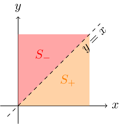
This integral requires some finesse to evaluate because of the absolute value. We will break the integral up into two integrals over different regions:
- \(\textcolor{red}{S_-} = \{ (x, y): x - y < 0 \}\)
- \(\textcolor{orange}{S_+} = \{ (x, y): x - y \geq 0 \}\)
in order to eliminate the absolute value. These two regions are shown in Figure 24.1.
Now, we can write \(|x - y|\) as \((x - y)\) on \(\textcolor{orange}{S_+}\) and \((y - x)\) on \(\textcolor{red}{S_-}\).
\[ \begin{aligned}
\text{E}\!\left[ |X - Y| \right] &= \iint_{\textcolor{orange}{S_+}} (x - y) \lambda_1 e^{-\lambda_1 x} \lambda_2 e^{-\lambda_2 y} \,dy\,dx + \iint_{\textcolor{red}{S_-}} (y - x) \lambda_1 e^{-\lambda_1 x} \lambda_2 e^{-\lambda_2 y} \,dy\,dx \\
&= \int_0^{\infty} \int_y^{\infty} (x - y) \lambda_1 e^{-\lambda_1 x} \lambda_2 e^{-\lambda_2 y} \,dx\,dy + \int_0^{\infty} \int_{x}^{\infty} (y - x) \lambda_1 e^{-\lambda_1 x} \lambda_2 e^{-\lambda_2 y} \,dy\,dx \\
&= \int_0^\infty \frac{1}{\lambda_1} e^{-\lambda_1 y} \lambda_2 e^{-\lambda_2 y} \,dy + \int_0^\infty \frac{1}{\lambda_2} e^{-\lambda_2 x} \lambda_1 e^{-\lambda_1 x} \,dx \\
&= \frac{\lambda_2}{\lambda_1} \frac{1}{\lambda_1+\lambda_2} + \frac{\lambda_1}{\lambda_2} \frac{1}{\lambda_1+\lambda_2} \\
&= \frac{\lambda_1^2 + \lambda_2^2}{\lambda_1\lambda_2(\lambda_1 + \lambda_2)}.
\end{aligned}
\]
Because Equation 24.1 is usually cumbersome to evaluate, 2D LotUS is usually a tool of last resort. The remainder of this chapter is devoted to shortcuts for specific functions \(g(x, y)\) that allow us to avoid 2D LotUS. But when in doubt, remember that 2D LotUS is always an option.
Linearity of Expectation
When \(g(x, y)\) is a linear function, there is a remarkable simplification.
Theorem 24.2 (Linearity of Expectation) Let \(X\) and \(Y\) be random variables. Then, \[
\text{E}\!\left[ X + Y \right] = \text{E}\!\left[ X \right] + \text{E}\!\left[ Y \right].
\]
Using 2D LotUS with \(g(x,y) = x + y\), we see that \[\begin{align*}
\text{E}\!\left[ X + Y \right] &= \int_{-\infty}^\infty \int_{-\infty}^\infty (x+y) \, f_{X,Y}(x,y) \, dx \, dy \\
&= \int_{-\infty}^\infty \int_{-\infty}^\infty x f_{X,Y}(x,y) \, dx \, dy + \int_{-\infty}^\infty \int_{-\infty}^\infty y f_{X,Y}(x,y) \, dx \, dy \\
&= \int_{-\infty}^\infty \int_{-\infty}^\infty xf_{X,Y}(x,y) \, dy \, dx + \int_{-\infty}^\infty \int_{-\infty}^\infty y f_{X,Y}(x,y) \, dx \, dy \\
&= \int_{-\infty}^\infty x \int_{-\infty}^\infty f_{X,Y}(x,y) \, dy \, dx + \int_{-\infty}^\infty y \int_{-\infty}^\infty f_{X,Y}(x,y) \, dx \, dy \\
&= \int_{-\infty}^\infty x f_X(x) \, dx + \int_{-\infty}^\infty y f_Y(y) \, dy \\
&= \text{E}\!\left[ X \right] + \text{E}\!\left[ Y \right].
\end{align*}\]
This result is more remarkable than it appears. It says that \(\text{E}\!\left[ X + Y \right]\), which depends in principle on the joint distribution of \(X\) and \(Y\), can be calculated using only the distribution of \(X\) and the distribution of \(Y\) individually. That is, no matter how \(X\) and \(Y\) are related to each other, \(\text{E}\!\left[ X + Y \right]\) is the same value.
By cleverly applying linearity of expectation, we can solve Example 24.1 without any double integrals!
Example 24.2 (How long does one person wait for the other? (Linearity Version)) In Example 24.1, we calculated \(\text{E}\!\left[ |X - Y| \right]\) using 2D LotUS. Of course, \(g(x, y) = |x - y|\) is not a linear function of \(x\) and \(y\), so we cannot apply linearity of expectation directly.
However, we can express the absolute difference \(|X - Y|\) as \(M - L\), where
- \(L \overset{\text{def}}{=}\min(X, Y)\) is the lesser of the two numbers (i.e., the time the first person enters), and
- \(M \overset{\text{def}}{=}\max(X, Y)\) is the greater of the two numbers (i.e., the time the second person enters).
Therefore, by linearity of expectation (Theorem 24.2),
\[ \text{E}\!\left[ |X - Y| \right] = \text{E}\!\left[ M - L \right] = \text{E}\!\left[ M \right] - \text{E}\!\left[ L \right], \] so we can evaluate the expectation by evaluating the expectations of \(M\) and \(L\) individually.
Determining \(\text{E}\!\left[ M \right]\) or \(\text{E}\!\left[ L \right]\) requires some work. To calculate \(\text{E}\!\left[ L \right]\), we will first need to calculate the distribution of \(L\). We will use the strategy from Section 20.1 and first calculate its CDF.
\[
\begin{align}
F_L(t) &= P(L \leq t) & \text{(definition of CDF)} \\
&= 1 - P(L > t) & \text{(complement rule)} \\
&= 1 - P(X > t, Y > t) & \text{(equivalent events)} \\
&= 1 - P(X > t) P(Y > t) & \text{(independence of $X$ and $Y$)} \\
&= 1 - (1 - F_X(t)) (1 - F_Y(t)) & \text{(write events in terms of CDF)} \\
&= 1 - e^{-\lambda_1 t} e^{-\lambda_2 t} & \text{(CDF of $X$ and $Y$)} \\
&= 1 - e^{-(\lambda_1 + \lambda_2) t}
\end{align}
\] for \(t \geq 0\).
If you do not recognize this CDF yet, take its derivative to obtain the PDF. \[
f_L(t) = \begin{cases} (\lambda_1 + \lambda_2) e^{-(\lambda_1 + \lambda_2) t} & t \geq 0 \\ 0 & \text{otherwise} \end{cases}.
\tag{24.2}\]
This is just the PDF of an \(\text{Exponential}(\lambda_1 + \lambda_2)\) random variable (Equation 22.2). Therefore, we know that \(\text{E}\!\left[ L \right] = \frac{1}{\lambda_1 + \lambda_2}\).
To calculate \(\text{E}\!\left[ M \right]\), we could follow the same process. (Exercise 24.1 asks you to work out the details.) However, once we know one of \(\text{E}\!\left[ M \right]\) or \(\text{E}\!\left[ L \right]\), we can determine the other using linearity of expectation.
First, observe that \(M + L\) is simply the sum of \(X\) and \(Y\) in some order; that is, \(M + L = X + Y\). Therefore, \[
\begin{aligned}
\text{E}\!\left[ M + L \right] &= \text{E}\!\left[ X + Y \right] \\
&= \text{E}\!\left[ X \right] + \text{E}\!\left[ Y \right] & \text{(linearity of expectation)} \\
&= \frac{1}{\lambda_1} + \frac{1}{\lambda_2} & \text{(expectation of exponential)}
\end{aligned}
\tag{24.3}\]
But again by linearity of expectation, \(\text{E}\!\left[ M + L \right] = \text{E}\!\left[ M \right] + \text{E}\!\left[ L \right]\), so Equation 24.3 us that \[ \text{E}\!\left[ M \right] + \text{E}\!\left[ L \right] = \frac{1}{\lambda_1} + \frac{1}{\lambda_2}. \] Since we already know that \(\text{E}\!\left[ L \right] = \frac{1}{\lambda_1 + \lambda_2}\), we can solve for the other expectation: \[
\text{E}\!\left[ M \right] = \frac{1}{\lambda_1} + \frac{1}{\lambda_2} - \frac{1}{\lambda_1 + \lambda_2}.
\]
Now we can simply subtract the two values to obtain \[
\begin{align}
\text{E}\!\left[ |X - Y| \right] = \text{E}\!\left[ M - L \right] = \text{E}\!\left[ M \right] - \text{E}\!\left[ L \right] &= \left(\frac{1}{\lambda_1} + \frac{1}{\lambda_2} - \frac{1}{\lambda_1 + \lambda_2} \right) - \frac{1}{\lambda_1 + \lambda_2} \\
&= \frac{\lambda_1^2 + \lambda_2^2}{\lambda_1\lambda_2(\lambda_1 + \lambda_2)},
\end{align}
\] which is the same answer as in Example 24.1 without any double integrals!
Expectation of Products
When \(g(x, y) = xy\), evaluating \(\text{E}\!\left[ g(X, Y) \right] = \text{E}\!\left[ XY \right]\) requires 2D LotUS in general. However, when \(X\) and \(Y\) are independent, we can break up the expectation.
Theorem 24.3 (Expectation of a product of independent random variables) If \(X\) and \(Y\) are independent random variables, then \[
\text{E}\!\left[ XY \right] = \text{E}\!\left[ X \right] \text{E}\!\left[ Y \right].
\] Moreover, for functions \(g\) and \(h\), \[
\text{E}\!\left[ g(X) h(Y) \right] = \text{E}\!\left[ g(X) \right] \text{E}\!\left[ h(Y) \right].
\]
Using 2D LotUS, we see that \[\begin{align*}
\text{E}\!\left[ XY \right] &= \int_{-\infty}^\infty \int_{-\infty}^\infty xy f_{X,Y}(x,y) \, dx \, dy \\
&= \int_{-\infty}^\infty \int_{-\infty}^\infty xy f_X(x) f_Y(y) \, dx \, dy & (\text{$X$ and $Y$ are independent}) \\
&= \int_{-\infty}^\infty y f_Y(y) \left[\int_{-\infty}^\infty x f_X(x) \, dx \right] \, dy & (\text{pull out constants with respect to $x$}) \\
&= \left[\int_{-\infty}^\infty x f_X(x) \, dx \right] \int_{-\infty}^\infty y f_Y(y) \, dy & (\text{pull out constants with respect to $y$}) \\
&= \text{E}\!\left[ X \right] \text{E}\!\left[ Y \right].
\end{align*}\]
The proof of the second part is similar.
Example 24.3 (Expected Product) Let \(X\) and \(Y\) be the waiting times of you and your friend, as in Example 23.7. Let \(L\) be the waiting time of the first person to enter and \(M\) be the waiting time of the second person to enter, as in Example 24.2.
What is \(\text{E}\!\left[ LM \right]\), the expected product of the two times?
We cannot apply Theorem 24.3 directly because \(L\) and \(M\) are not independent. If we know that the first person waited \(L = 5\) minutes, then the second person cannot have waited less than that.
However, we can observe that \(LM\) is simply the product of the two waiting times \(X\) and \(Y\) in some order. That is, \(LM = XY\), where \(X\) and \(Y\) are independent. Therefore, \[
\text{E}\!\left[ LM \right] = \text{E}\!\left[ XY \right] = \text{E}\!\left[ X \right] \text{E}\!\left[ Y \right] = \frac{1}{\lambda_1} \frac{1}{\lambda_2} = \frac{1}{\lambda_1\lambda_2}.
\]
On the other hand, we calculated \(\text{E}\!\left[ L \right]\) and \(\text{E}\!\left[ M \right]\) in Example 24.2, and \[ \text{E}\!\left[ L \right] \text{E}\!\left[ M \right] = \left( \frac{1}{\lambda_1 + \lambda_2} \right) \left( \frac{1}{\lambda_1} + \frac{1}{\lambda_2} - \frac{1}{\lambda_1 + \lambda_2} \right) \neq \text{E}\!\left[ LM \right]. \]
Why should we care about \(\text{E}\!\left[ LM \right]\), the expected product of these two waiting times? It turns out to be useful for summarizing the relationship between \(L\) and \(M\). We take up this issue in Chapter 25.
Exercises
Exercise 24.1 In Example 24.2, we derived the PDF of \(L = \min(X, Y)\), the waiting time of the first person to enter. Using a similar argument, derive the PDF of \(M = \max(X, Y)\), the waiting time of the second person to enter. Then, using this PDF, calculate \(\text{E}\!\left[ M \right]\), and check that it matches the answer we obtained in Example 24.2.