12 Named Distributions

So far, we have encountered distributions which arise so commonly that they have names such as Bernoulli, binomial, and geometric. In this section, we review these named distributions and introduce a few more. This chapter is also intended to be a useful reference, compiling the properties of these named distributions in a single place.

12.1 Bernoulli and Binomial Distributions

We introduced the Bernoulli and binomial distributions in Section 8.4. A Bernoulli random variable represents the outcome of a single toss of a possibly biased coin ($1$ if heads, $0$ if tails), while a binomial random variable represents the number of heads in $n$ tosses of the same coin.

We recall the definitions and properties we derived earlier.

Definition 8.6 (Binomial distribution)

If $X$ is a random variable with PMF \[ f(x) = \binom{n}{x} p^x (1-p)^{n-x};\qquad x = 0, 1, \dots, n \tag{12.1}\] for some $n$ and $0 < p < 1$, $X$ is said to be a binomial random variable with parameters $n$ and $p$. We write this as $X \sim \text{Binomial}(n,p)$.

A Bernoulli random variable is simply a $\text{Binomial}(n=1, p)$ random variable. We argued in Example 10.6 that if $X_1, X_2, \dots, X_n$ are independent $\text{Bernoulli}(p)$ random variables, then \[ T_n \overset{\text{def}}{=}X_1 + X_2 + \dots + X_n \sim \text{Binomial}(n, p). \]

Next, we calculate the expectation and variance of a binomial random variable.

Proposition 9.2 and Proposition 11.3 (Binomial expectation and variance)

Let $X \sim \text{Binomial}(n,p)$. Then, \[\text{E}\!\left[ X \right] = np\] and \[\text{Var}\!\left[ X \right] = np(1 - p).\]

Since a Bernoulli random variable is simply a $\text{Binomial}(n=1, p)$ random variable, its expectation and variance are $p$ and $p(1 - p)$, respectively.

We have encountered many examples of binomial distributions already, including Example 8.8 and Example 8.9; the next example presents another scenario that arises in manufacturing.

Example 12.1 (Sampling with replacement) Quality control is essential in manufacturing. For example, a factory that manufactures cans might want to ensure that the cans do not have dents or other defects.

Suppose the factory manufactures $N$ cans in each lot. It may be impractical to inspect all $N$ cans, in which case the factory randomly selects $n$ items and inspects them. If there are $c$ or more defective items in the sample, the lot is rejected.

Assume there are $M$ defective cans in a lot, and a sample of $n$ cans is taken with replacement. That is, each time a can is inspected, it is put back into the lot before another can is selected for inspection. This means that there is a chance that the same can may be inspected more than once.

If $X$ is the number of defective cans in the sample, then $X$ is a random variable that assumes values from $0$ to $n$. Each selected can has a probability $p = \frac{M}{N}$ of being defective, and because the cans are replaced, the selected cans are independent. Therefore, $X$ is a $\text{Binomial}(n, p=\frac{M}{N})$ random variable.

Now, we can use known facts about the binomial distribution. For example, the probability that the lot is rejected is \[ P(X \geq c) = \sum_{x=c}^n f_X(x) = \sum_{x=c}^n \binom{n}{x} \Big(\frac{M}{N}\Big)^x \Big(1 - \frac{M}{N}\Big)^{n-x}, \] and the expected number of defects in the sample is \[ \text{E}\!\left[ X \right] = n \frac{M}{N}. \]

To make this example concrete, suppose that a lot consists of $N = 2000$ cans, of which $M = 150$ are defective. The factory randomly samples $n = 60$ cans for inspection. The lot is rejected if $c = 5$ or more cans in the sample are defective.

To evaluate the probability that the lot is rejected, it is easier to use R than to calculate it by hand. One of the benefits of working with named distributions is that their PMFs and CDFs are built into R. In general, R has functions called dNAME and pNAME for the PMF and CDF, respectively, of every named distribution (where NAME identifies the distribution, such as binom or geom).

12.2 Hypergeometric Distribution

In Example 12.1, we assumed that cans were selected with replacement. However, in quality control, the inspected items are usually selected without replacement. This may be because the inspection process itself is destructive (e.g., crash tests for a car). But even if the inspection process is not destructive, it seems redundant to inspect the same item twice. For this reason, in quality control (and in statistics more generally), most sampling is done without replacement. A sample that is collected by sampling without replacement from a population, where every unit is equally likely to be in the sample, is called a simple random sample.

If $n$ cans are sampled without replacement from a lot of $N$ cans, where $M$ are defective, then the number of defective cans in the sample $X$ is said to be a $\text{Hypergeometric}(n, M, N)$ random variable.

What is the PMF of $X$? In other words, what is $P(X = x)$, the probability that exactly $x$ cans are defective? We cannot use the binomial formula because each draw affects subsequent draws; this is not analogous to $n$ tosses of a coin because the probability of “heads” is changing with each toss. In order to calculate this probability, we resort to counting.

How many possible outcomes are there? In Chapter 2, we saw that the number of distinct ways to select $n$ items from $N$ items, ignoring order, is $\binom{N}{n}$.
How many outcomes are in the event $\{ X = x \}$? There are $\binom{M}{x}$ ways to choose $x$ defective cans and $\binom{N - M}{n - x}$ ways to choose the remaining $n - x$ non-defective cans. By Theorem 2.1, the number of possible ways to choose $x$ defective and $n - x$ non-defective cans is $\binom{M}{x} \binom{N - M}{n - x}$.

Putting the pieces together, we obtain the PMF of a $\text{Hypergeometric}(n, M, N)$ random variable.

Definition 12.1 (Hypergeometric distribution) If $X$ is a random variable with PMF \[ f(x) = \frac{\displaystyle \binom{M}{x} \binom{N - M}{n - x}}{\displaystyle \binom{N}{n}}; \qquad x = 0, 1, \dots, \min(n, M), \tag{12.2}\] for positive integers $n, M < N$, then we say that $X$ is a hypergeometric random variable with parameters $n$, $M$, and $N$. We write this as $X \sim \text{Hypergeometric}(n, M, N)$.

Next, we present formulas for the expected value and variance of the hypergeometric distribution.

Proposition 12.1 (Hypergeometric expectation and variance) Let $X$ be a $\text{Hypergeometric}(n, M, N)$ random variable. Then:

\[ \begin{align} \text{E}\!\left[ X \right] &= n \frac{M}{N} & \text{Var}\!\left[ X \right] &= n \frac{M}{N} \left(1 - \frac{M}{N}\right) \frac{N - n}{N - 1} \end{align} \]

Proof

Since calculating the expectation and variance requires calculating $\text{E}\!\left[ X \right]$ and $\text{E}\!\left[ X^2 \right]$, we will start by deriving a general formula for the $k$th moment $\text{E}\!\left[ X^k \right]$ for $k \geq 1$.

\[\begin{align*} \text{E}\!\left[ X^k \right] &= \sum_{x=0}^n x^k \frac{\binom{M}{x} \binom{N - M}{n-x}}{\binom{N}{n}} & \text{(LotUS)} \\ &= M \sum_{x=1}^n x^{k-1} \frac{\binom{M - 1}{x-1} \binom{N - M}{n-x}}{\binom{N}{n}} & \left( x\binom{M}{x} = M\binom{M-1}{x-1} \right) \\ &= n\frac{M}{N} \sum_{x=1}^n x^{k-1} \frac{\binom{M - 1}{x-1} \binom{N - M}{n-x}}{\binom{N - 1}{n - 1}} & \left( \binom{N}{n} = \frac{N}{n} \binom{N - 1}{n - 1} \right) \\ &= n\frac{M}{N} \sum_{i=0}^{n-1} (i+1)^{k-1} \frac{\binom{M-1}{i} \binom{N - M}{n-1-i}}{\binom{N - 1}{n-1}} & \left(i = x - 1 \right) \\ &= n\frac{M}{N} \text{E}\!\left[ (Y+1)^{k-1} \right] & \text{(LotUS)}, \end{align*}\] where $Y \sim \text{Hypergeometric}(n-1, M-1, N)$.

Setting $k = 1$, we obtain \[ \text{E}\!\left[ X \right] = n\frac{M}{N} \text{E}\!\left[ (Y + 1)^0 \right] = n\frac{M}{N}, \] and setting $k=2$, we obtain \[ \begin{aligned} \text{E}\!\left[ X^2 \right] &= n\frac{M}{N} \text{E}\!\left[ (Y+1)^1 \right] \\ &= n\frac{M}{N} \left( (n - 1) \frac{M - 1}{N - 1} + 1 \right). \end{aligned} \] Thus, the variance is \[ \begin{aligned} \text{Var}(X) &= \text{E}\!\left[ X^2 \right] - \text{E}\!\left[ X \right]^2 \\ &= n \frac{M}{N} \left( (n-1)\frac{M-1}{N - 1} + 1 - n\frac{M}{N} \right) \\ &= n \frac{M}{N} \left( \frac{(n-1)(M - 1) N + N(N-1) - nM (N-1)}{N(N - 1)} \right) \\ &= n \frac{M}{N} \left(\frac{-nN - MN + N^2 + nM}{N(N-1)} \right) \\ &= n \frac{M}{N} \frac{N - M}{N} \frac{N - n}{N - 1}. \end{aligned} \]

If we let $p \overset{\text{def}}{=}\frac{M}{N}$ be the probability that each selected can is defective, then the expected value of the hypergeometric distribution is the same as that of the binomial, but the variance becomes $np(1 - p)\frac{N - n}{N - 1}$, which differs from the binomial by a factor of $\frac{N - n}{N - 1}$.

We compare the binomial and hypergeometric distributions in the next example.

Example 12.2 (Simple random sample) Consider Example 12.2, with a lot of $N = 2000$ cans, of which $M = 150$ are defective. However, assume that the $n = 60$ cans are sampled without replacement. What is the probability now that the lot is rejected?

If $X$ represents the number of defective cans in the sample, then $X$ is a $\text{Hypergeometric}(n=60, M=150, N=2000)$ random variable. The probability $P(X \geq 5)$ that the lot is rejected can be calculated as \[ \sum_{x=5}^{60} \frac{\binom{150}{x} \binom{1850}{60-x}}{\binom{2000}{60}}, \] which is best evaluated using R.

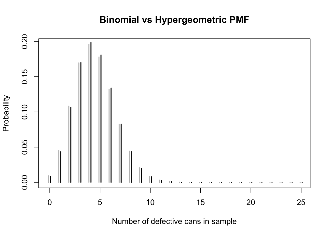
This probability is very close to the probability we obtained in Example 12.2, when the cans were sampled with replacement. This is no accident. The two PMFs are graphed in Figure 12.1. The hypergeometric (in black) has slightly more mass in the center, near the expected value of $n\frac{M}{N} = 4.5$, while the binomial (in gray) has slightly more mass in the tails. This is because when cans are sampled without replacement, each time a defective can is sampled, the probability of sampling another defective decreases. Therefore, extreme numbers of defective cans are less likely when sampling without replacement.

Figure 12.1: Hypergeometric (in black) vs. Binomial (in gray) PMFs for $x = 0, 1, \dots, 25$. The remaining probabilities are negligible.

The fact that the hypergeometric has less mass in the tails than the binomial is reflected in the variances of the two distribution. The hypergeometric variance differs from the binomial variance by a factor of $\frac{N - n}{N - 1}$. For this example, the factor is \[ \frac{N - n}{N - 1} = \frac{2000 - 100}{2000 - 1} \approx .95, \] only a little bit less than $1.0$, which again reinforces the fact that the distributions are quite similar.

In general, when the sample size $n$ is much smaller than the lot size $N$, this factor will be close to $1.0$, and the hypergeometric and binomial distributions will be quite similar. For this reason, when the population size $N$ is very large relative to the sample size $n$, it is typical to use the binomial distribution, even if the sampling is done without replacement.

In fact, if the lot size $N$ were infinite, then there would be no difference between sampling with and without replacement because the probability of sampling the same can twice would be zero! In other words, the binomial distribution is like the hypergeometric distribution with an infinite population. For this reason, the extra factor of $\frac{N - n}{N - 1}$ in the hypergeometric variance is called the finite population correction.

The hypergeometric distribution is also useful in other contexts, as the next two examples show.

Example 12.3 (Mark-Recapture)

How can we estimate the size of a population, such as the number of a snails in a state park? There may be too many to count, and it may be difficult to catch them all. Another way is mark-recapture. First, we capture a sample, say $50$ snails, and “mark” them, as shown at right.

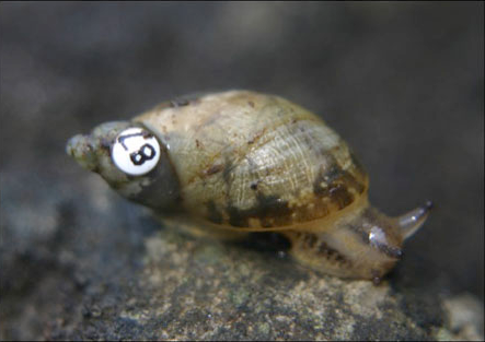
Then, after some time has elapsed, we recapture another sample of snails, say $40$. Some of these snails will be marked from the first capture, while the rest are unmarked. The number of recaptured snails that are marked can be used to estimate the number of snails in the population. In Chapter 29, we will see how to use this data to estimate the number of snails in the population.

For now, we will assume that there are actually $300$ snails in the population. What is the probability that exactly $11$ marked snails are recaptured in the second sample of $40$ snails?

If every snail in the population has an equal chance of being sampled, then the “recapture” is exactly like a sample of cans in a lot. The marked snails are $M = 50$ defective cans out of $N = 300$ cans total, and we are recapturing $n = 40$ distinct snails (i.e., without replacement) from the population.

Therefore, the number of marked snails in the second sample, $X$, is a $\text{Hypergeometric}(n=40, M=50, N=300)$ random variable, so the probability of exactly $11$ marked snails can be obtained by substituting $x = 11$ into the hypergeometric PMF (Equation 12.2): \[ P(X = 11) = \frac{\binom{50}{11} \binom{300 - 50}{40 - 11}}{\binom{300}{40}} \approx .0276. \]

We can also use R to evaluate this probability. Note that the parameters of the hypergeometric in R are $M$, $N - M$, and $n$, in that order.

Example 12.3 is unrealistic. If we knew that there were $N = 300$ snails in the population, then there would be no reason to do mark-recapture in the first place! In Chapter 29, we will revisit this example and answer the more realistic (and statistical) question of how to estimate the population size $N$ from observed data, such as $X = 11$.

Example 12.4 (Lady Tasting Tea)

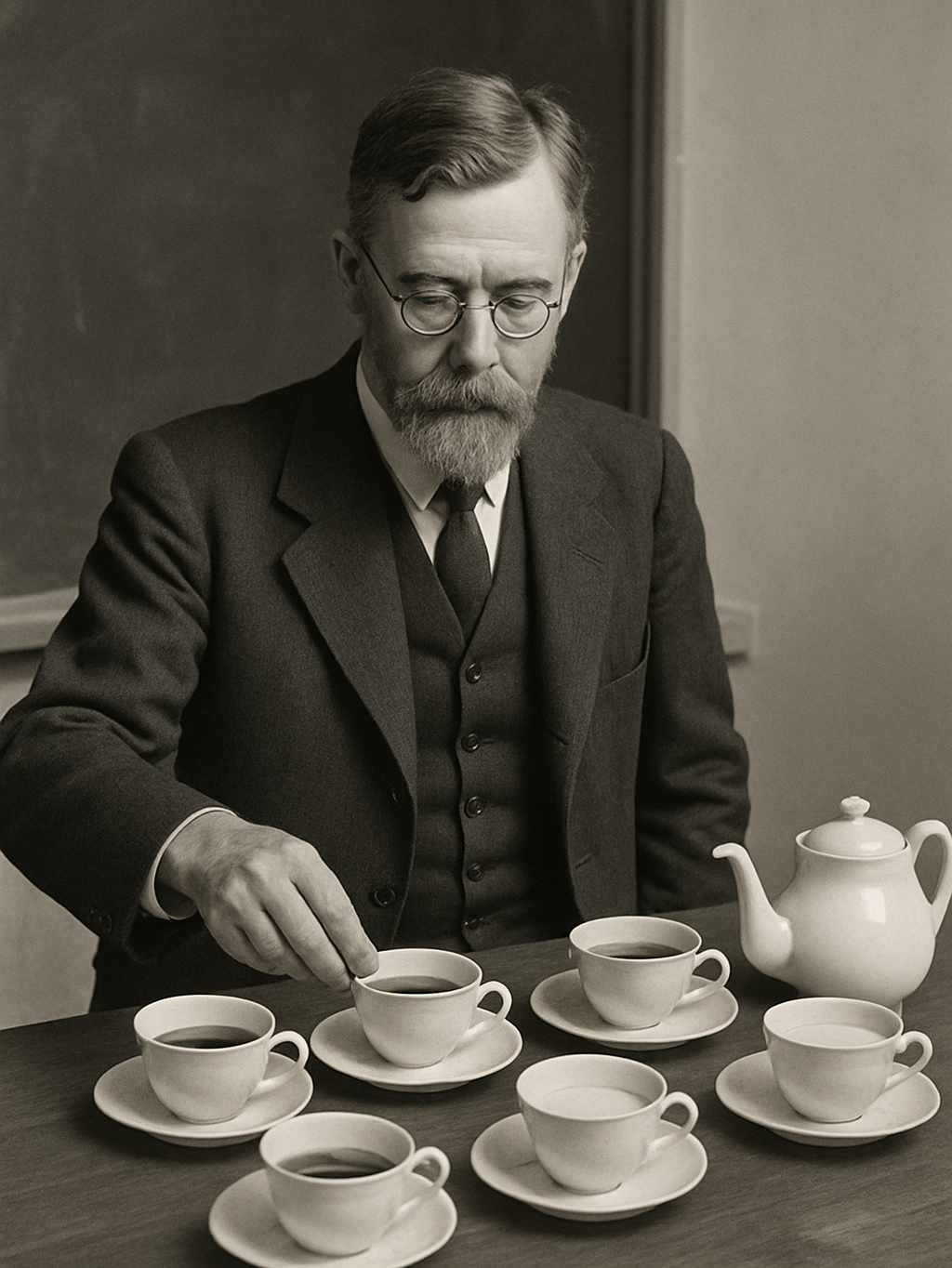
One afternoon, the English statistician and geneticist R. A. Fisher poured a cup of tea, added milk, and offered it to the lady sitting beside him, the ecologist Muriel Bristol. She refused the tea, saying that she preferred tea when the milk was poured first. Fisher did not believe that it could possibly make any difference, so he set up an experiment to test her claim.

He prepared $8$ cups of tea, $4$ with milk poured first and $4$ with tea poured first. He then mixed them up and asked Bristol to identify which cups had the milk poured first. She correctly identified all $4$ cups.

An artist’s rendition of the Lady Tasting Tea experiment

Fisher took this as convincing evidence that Bristol could tell the difference. Here was his argument. First, he assumed that she could not tell the difference and was merely guessing. Fisher called this assumption the “null hypothesis”. If this were the case, then the $4$ cups she picked might as well be a random sample from the $8$ cups.

In other words, the cups with milk poured first are like $M = 4$ defective cans from a lot of $N = 8$ cans. If the null hypothesis were true, then the cups that Bristol picked would be like a random sample of $n = 4$ cans without replacement. Therefore, under the null hypothesis, the number of cups with milk poured first that she correctly identified, $X$, is a $\text{Hypergeometric}(n=4, M=4, N=8)$ random variable.

In fact, Bristol identified $X = 4$ of the cups correctly. The probability of this under the null hypothesis is \[ P(X = 4) = \frac{{4 \choose 4} {4 \choose 0}}{{8 \choose 4}} = \frac{1}{70} \approx .0143. \]

Because this probability (which Fisher called the “p-value”) is very small, Fisher rejected the null hypothesis that she was just guessing and concluded that Bristol could tell the difference after all.

Today, the hypothesis test that Fisher carried out in Example 12.4, based on the hypergeometric distribution, is called Fisher’s exact test in his honor. We will discuss hypothesis testing more fully in Chapter 46.

12.3 Geometric and Negative Binomial Distributions

In Section 8.5, we defined a $\text{Geometric}(p)$ random variable, which counts the number of coin tosses until we observe “heads” for the first time. We argued that its PMF is \[ f(n) = (1-p)^{n-1} p; \quad n = 1, 2, \dots \] because in order for the first “heads” to be on toss $n$, the first $n-1$ tosses must all be “tails”.

We can generalize the geometric distribution. Let $X$ count the number of tosses of a coin (with probability $p$ of “heads”) until we have observed $r$ “heads” in total. Then, $X$ is said to be a negative binomial random variable. Notice that the geometric distribution corresponds to the special case $r = 1$.

What is the PMF of $X$? Let’s build intuition by looking at a specific case. Suppose we want to know the probability that it takes exactly 5 tosses to observe 3 “heads”. That is, we want to calculate $P(X = 5)$, where $X \sim \text{NegativeBinomial}(r=3, p)$. Here are all the possible sequences where the 3rd “heads” happens on the 5th toss:

HHTTH
HTHTH
HTTHH
THHTH
THTHH
TTHHH

Each sequence consists of exactly 3 “heads” and 2 “tails”, so they all have the same probability, \[ p^3 (1-p)^2. \]

Therefore, the overall probability is this probability multiplied by the number of such sequences, which in this case is $6$. To count the number of sequences without listing them all, we can reason as follows:

In order for the 3rd “heads” to occur on the 5th toss, the last toss must be H. (If the sequence were instead something like HHTHT, the 3rd “heads” would be on the 4th toss, not the 5th.)
Since the last toss must be H, this leaves $3 - 1 = 2$ “heads” to arrange among the remaining $5 - 1 = 4$ tosses.
The number of such sequences is therefore $\binom{4}{2} = 6$.

We can generalize this argument to any number of “heads” $r$ and any probability $P(X = x)$. In this way, we obtain a general formula for the PMF of a negative binomial random variable.

Definition 12.2 (Negative binomial distribution) If $X$ is a random variable with PMF \[ f(x) = \binom{x-1}{r-1} p^r (1-p)^{x-r}; \qquad x = r, r+1, \dots \tag{12.3}\] for some positive integer $r$ and $0 < p < 1$, we say that $X$ is a negative binomial random variable with parameters $r$ and $p$. We write this as $X \sim \text{NegativeBinomial}(r,p)$.

If we plug in $r = 1$ into Equation 12.3, we obtain \[ f(x) = \binom{x - 1}{0} p^1 (1 - p)^{x - 1} = (1 - p)^{x-1} p; \quad x = 1, 2, \dots, \] which is precisely the PMF for a $\text{Geometric}(p)$ random variable.

We can also derive formulas for the expected value and variance.

Proposition 12.2 (Negative binomial expectation and variance) \[ \begin{align} \text{E}\!\left[ X \right] &= \frac{r}{p} & \text{Var}\!\left[ X \right] &= \frac{r(1-p)}{p^2} \end{align} \]

Proof

Let $X \sim \text{NegativeBinomial}(r,p)$. Then, \[\begin{align*} \text{E}\!\left[ X^k \right] &= \sum_{x=r}^\infty x^k \binom{x-1}{r-1} p^r (1-p)^{x-r} & \text{(LotUS)}\\ &= \sum_{x=r}^\infty x^{k-1} r \binom{x}{r} p^r (1-p)^{x-r} & \left( x \binom{x - 1}{r - 1} = r \binom{x}{r} \right) \\ &= r \sum_{i=r + 1}^\infty (i - 1)^{k-1} \binom{i - 1}{r} p^r (1-p)^{i-1-r} & \left( i = x + 1 \right) \\ &= \frac{r}{p} \sum_{i=r + 1}^\infty (i - 1)^{k-1} \underbrace{\binom{i - 1}{(r + 1) - 1} p^{r + 1} (1-p)^{i-(r + 1)}}_{\text{NegativeBinomial}(r+1, p) \text{ PMF}} & \text{(rewrite in terms of $r + 1$)} \\ &= \frac{r}{p} \text{E}\!\left[ (Y-1)^{k-1} \right] & \text{(LotUS)}, \end{align*}\] where $Y \sim \text{NegativeBinomial}(r+1, p)$.

Setting $k=1$, we get \[ \text{E}\!\left[ X \right] = \frac{r}{p} \text{E}\!\left[ (Y - 1)^0 \right] = \frac{r}{p}, \] and setting $k = 2$, we get \[ \text{E}\!\left[ X^2 \right] = \frac{r}{p} \text{E}\!\left[ (Y-1)^1 \right] = \frac{r}{p} \left( \frac{r+1}{p} - 1 \right). \] Thus, \[ \text{Var}\!\left[ X \right] = \text{E}\!\left[ X^2 \right] - \text{E}\!\left[ X \right]^2 = \frac{r}{p}\left( \frac{r+1}{p} - 1 - \frac{r}{p} \right) = \frac{r(1-p)}{p^2}. \]

Notice that if we substitute $r = 1$ into the expectation, we obtain $\text{E}\!\left[ X \right] = \frac{1}{p}$, which we previously derived in Example 9.7. However, we now also see that the variance of the geometric distribution is $\text{Var}\!\left[ X \right] = \frac{1 - p}{p^2}$.

Example 12.5 (Number of interviews) A medical researcher needs to recruit 20 subjects for a clinical trial. Each person she interviews has a 60% chance of being eligible to participate in the study, independently of any other subject.

How many people should she expect to interview?
What is the probability she will have to interview at least 40 people?

If $X$ is the number of interviews required, then $X \sim \text{NegativeBinomial}(r=20, p=0.60)$. To convince ourselves, we make an analogy with coin tosses.

Each coin toss represents a person that she interviews.
A “heads” means that the person is eligible.
She will toss the coin until she gets $r = 20$ “heads.”
$X$ counts the number of tosses.

Therefore, the expected number of people she has to interview is \[ \text{E}\!\left[ X \right] = \frac{r}{p} = \frac{20}{0.6} \approx 33.33, \] and the probability is \[ P(X \geq 40) = \sum_{k = 40}^\infty \binom{k-1}{19} (0.6)^{20} (0.4)^{k-20}. \]

To avoid an infinite sum, we can use the complement rule: \[ P(X \geq 40) = 1 - P(X \leq 39) = 1 - \sum_{k = 20}^{39} \binom{k-1}{19} (0.6)^{20} (0.4)^{k-20}. \]

But this sum is still impractical to evaluate by hand. We can use dnbinom in R to evaluate this probability. Note that R uses a different definition of a negative binomial random variable that counts only the “tails”, rather than the total number of tosses. To convert our value into the number of tails, we need to subtract the $r = 20$ “heads” from the value we plug into R.

12.4 Poisson Distribution

Imagine that you are in a room of $n$ people, including yourself. Each person in the room has contributed $1 to a central pot, so there is a total of $$n$ in the pot. The money in the pot will be redistributed back to the people in the room as follows: each dollar is equally likely to go to any one of the $n$ people, independently of the other dollars in the pot. Some people will end up with more than $1, while others end up with nothing.

As $n \to \infty$, what is the probability you end up with nothing? There are two lines of reasoning that lead to contradictory answers:

As $n \to \infty$, the number of dollars in the pot goes to infinity, so it seems that the probability that you end up with at least one of these infinite dollars should approach $1$; i.e., the probability that you end up with nothing is $0$.
As $n \to \infty$, the chance that you earn each dollar, $1/n$, decreases to $0$. So it seems that the probability that you end up with nothing is $1$.

Which line of reasoning is correct? It turns out that both are wrong!

We can solve this problem using the binomial distribution.

Example 12.6 (Ending up with zero dollars) Each of the $n$ dollars has a probability of $1/n$ of being returned to you. So, if $X$ is the number of dollars we get, then $X \sim \text{Binomial}(n,1/n)$. The probability we get zero dollars is \[ f_X(0) = \binom{n}{0} \left( \frac{1}{n} \right)^0 \left( 1 - \frac{1}{n} \right)^{n} = \left( 1 - \frac{1}{n} \right)^n. \] From calculus, we know that \[ \lim_{n \to \infty} \left( 1 - \frac{1}{n} \right)^n = e^{-1}. \]

Deriving the limit

Here’s one way to establish the limit. Replace the integer $n$ by $1 / x \in \mathbb{R}$, and take the limit as $x \to 0$: \[ \lim_{n \to \infty} \left( 1 - \frac{1}{n} \right)^n = \lim_{x \to 0} \left( 1 - x \right)^{1/x}, \] and observe that this limit has indeterminate form $1^\infty$. We can determine the limit by applying L’Hopital’s rule to the logarithm: \[ \lim_{x\to 0 } \ln ( 1 - x )^{1/x} = \lim_{x\to 0} \frac{\ln(1 - x)}{x} = \lim_{x\to 0} \frac{-\frac{1}{1 - x}}{1} = -1. \]

Since the limit of the (natural) logarithm is $-1$, the limit of the original expression must be $e^{-1}$.

It turns out that the above phenomenon is not a coincidence. In general, a binomial distribution with large $n$ and small $p$ can be approximated by a PMF involving the number $e$.

Theorem 12.1 (Poisson approximation to the binomial) Let $X \sim \text{Binomial}(n,p = \mu/n)$, where $\mu$ is a constant. Then, the PMF of $X$ approaches \[ f(x) = e^{-\mu} \frac{\mu^x}{x!}; \qquad x = 0,1,2, \dots \] as $n \to \infty$.

Proof

Let $X \sim \text{Binomial}(n, p = \mu/ n)$. Then its PMF is \[ f(x) = \binom{n}{x} \left( \frac{\mu}{n} \right)^x \left( 1 - \frac{\mu}{n} \right)^{n-x}. \]

Now, we regroup this expression into four terms \[ \begin{aligned} f(x) &= \underbrace{\frac{\mu^x}{x!}}_{\text{(a)}} \cdot \underbrace{\frac{n!}{(n-x)! n^x}}_{\text{(b)}} \cdot \underbrace{\left(1 - \frac{\mu}{n}\right)^n}_{\text{(c)}} \cdot \underbrace{\left(1 - \frac{\mu}{n}\right)^{-x}}_{\text{(d)}}, \end{aligned} \] and take the limit of each of these terms as $n \to \infty$:

$\frac{\mu^x}{x!}$ does not depend on $n$ so it is constant.
$\frac{n!}{(n-x)! n^x}$ can be expanded as $\frac{n(n-1)\dots (n-x+1)}{n^x}$. There are $x$ terms in the numerator and $x$ terms in the denominator. The terms in the numerator are close to $n$ when $n$ is large, so the limit is $1$.
$\left(1 - \frac{\mu}{n}\right)^n \to e^{-\mu}$, as discussed in Example 12.6.
$\left(1 - \frac{\mu}{n}\right)^{-x} \to 1^{-x} = 1$, since $\frac{\mu}{n} \to 0$.

Note that we can apply Theorem 12.1 to Example 12.6 by taking $\mu = 1$. Theorem 12.1 says that the probability is approximately \[ f(0) = e^{-1} \frac{1^0}{1!} = e^{-1}, \] which matches the answer we got in Example 12.6.

Theorem 12.1 motivates the following named distribution.

Definition 12.3 (Poisson distribution) If $X$ is a random variable with PMF \[ f(x) = e^{-\mu} \frac{\mu^x}{x!}; \qquad x = 0,1,2, \dots \] for some $\mu > 0$, we say that $X$ is a Poisson random variable with parameter $\mu$. We denote it by $X \sim \text{Poisson}(\mu)$.

Next, we derive the expectation and variance for a Poisson random variable. Since the Poisson distribution is an approximation to a $\text{Binomial}(n, p=\frac{\mu}{n})$ distribution, we might conjecture that the Poisson expectation is \[ \text{E}\!\left[ X \right] = np = n\frac{\mu}{n} = \mu. \] This intuition turns out to be correct, but this fact requires proof.

Proposition 12.3 (Poisson expectation and variance) Let $X \sim \text{Poisson}(\mu)$. Then, \[ \begin{aligned} \text{E}\!\left[ X \right] &= \mu & \text{Var}\!\left[ X \right] &= \mu \end{aligned} \]

Proof

We derive a general formula for $\text{E}\!\left[ X^k \right]$ for $k \geq 1$.

\[ \begin{align} \text{E}\!\left[ X^k \right] &= \sum_{x=0}^\infty x^k e^{-\mu} \frac{\mu^x}{x!} & \text{(LotUS)} \\ &= \sum_{x=1}^\infty x^k e^{-\mu} \frac{\mu^x}{x!} & \text{($x=0$ term is zero)} \\ &= \sum_{x=1}^\infty x^{k-1} e^{-\mu} \frac{\mu^x}{(x-1)!} & \text{(cancel $x$ with one factor of $x!$)} \\ &= \sum_{i=0}^\infty (i + 1)^{k-1} e^{-\mu} \frac{\mu^{i+1}}{i!} & (i = x - 1) \\ &= \mu \sum_{i=0}^\infty (i + 1)^{k-1} \underbrace{e^{-\mu} \frac{\mu^i}{i!}}_{\text{$\text{Poisson}(\mu)$ PMF}} \\ &= \mu \text{E}\!\left[ (X + 1)^{k-1} \right]. & \text{(LotUS)} \end{align} \]

Setting $k=1$, we obtain the expectation that we conjectured, \[ \text{E}\!\left[ X \right] = \mu \text{E}\!\left[ (X + 1)^{0} \right] = \mu. \]

To obtain the variance, we first set $k=2$ to obtain $\displaystyle \text{E}\!\left[ X^2 \right] = \mu \text{E}\!\left[ (X + 1)^{1} \right] = \mu (\mu + 1)$. Therefore, \[ \text{Var}\!\left[ X \right] = \text{E}\!\left[ X^2 \right] - \text{E}\!\left[ X \right]^2 = \mu( \mu + 1 - \mu) = \mu. \]

The next example shows a natural situation where the Poisson distribution arises.

Example 12.7 (Detecting Radiation) A Geiger counter is a device that measures the level of ionizing radiation. It makes a clicking sound each time an ionization event is detected. In each millisecond, there is a small probability $p = 1 / 50000$ of a click. If we assume that milliseconds are independent, then the number of clicks over one minute is \[ X \sim \text{Binomial}(n=60000, p=1/50000) \approx \text{Poisson}(\mu=np=1.2). \]

What is the probability that there is more than 1 click over this minute?

\[ P(X > 1) = 1 - P(X = 0) - P(X = 1) = 1 - e^{-1.2} \frac{1.2^0}{0!} - e^{-1.2} \frac{1.2^1}{1!} \approx .3373. \]

We could use R to calculate this probability and the exact binomial probability.

The Poisson approximation is accurate to over 5 decimal places! Because the Poisson distribution only requires specifying the overall rate $\mu$, rather than $n$ and $p$, it is often more convenient than the binomial distribution.

In Example 12.7, the clicks of the Geiger counter happen at random times. The times at which these clicks occur constitute a random process called a Poisson process because the number of clicks over any time interval is a Poisson random variable. We will revisit Poisson processes in Section 18.3.

12.5 Exercises

Exercise 12.1 (Cardano’s example revisited) Recall Solution 2.1, where Cardano was interested in how many rolls of a fair die are necessary in order to have at least even odds of one or more sixes?

In other words, we need to derive an expression for $P(\text{at least one six in $n$ rolls})$.

Define a binomial random variable $X$ and express the probability above in terms of $X$.
Define a negative binomial random variable $Y$ and express the probability above in terms of $Y$.
Use either named distribution above to calculate the probability.

Exercise 12.2 (Overselling) Have you ever been offered money by an airline to take a later flight? This is because airlines often oversell tickets. For example, if there are only 162 seats on a plane, they may sell 170 tickets for a flight, expecting that some passengers will be no-shows.

The airline loses money if more than 162 passengers show up and demand compensation for being moved to another flight. But an airline also loses money if they fly the plane with empty seats when there are people who would have gladly paid for those seats.

Suppose that an airline sells 170 tickets for a flight with 162 tickets, and each passenger has a 95% probability for showing up for a flight. What is the probability that the flight is oversold? That is, more people show up than there are seats on the flight.

Exercise 12.3 (Flush in Texas Hold’em) Texas Hold’em is a popular variant of poker. First, each player is dealt two cards of their own. Then, five “community” cards are dealt in the center of the table. The player wins if they have the best poker hand among the seven cards (the two cards in their hand, plus the five community cards shared by all the players).

Let’s say you are dealt the following cards:

Ace of spades
9 of spades.

With two spades already in hand, you might hope for a flush of spades, which requires five total spades.

Define a random variable $X$ which follows one of the named distributions in this chapter, and express the probability of a flush in terms of $X$. Then, calculate the probability of a flush.

Exercise 12.4 (Error correcting codes) Files on your computer are encoded as a sequence of 0s and 1s. Each 0 or 1 is called a bit.

For example, a 1 KB file consists of 8,192 0s and 1s. (That’s because there are 1,024 bytes in a KB and 8 bits in a byte, so a 1 KB file contains 8,192 bits.)

Sometimes, bits get corrupted in transit. So a 0 might get changed to a 1, or vice versa.

Suppose that we download a 1 KB file using a connection where each bit has a $.0003$ probability of being corrupted, independently of any other bit.

What is the probability that at least one bit is corrupted?
To detect if a file has been corrupted, files will sometimes contain an extra bit appended to the end, called the checksum. This extra bit is 1 if there should be an odd number of 1s in the message (i.e., the main body of the file) and 0 if there should be an even number. If there is a mismatch, then we know that the file is corrupted. What is the probability that at least one bit is corrupted and this is not caught by the checksum?

Exercise 12.5 (Fair coin from unfair coin revisited) In Exercise 6.1, we discussed one way to simulate a fair coin using an unfair coin with probability $p \neq .5$ of landing heads. Flip the coin twice: if the two flips are different, then consider HT as heads and TH as tails. In Exercise 6.1, you showed that these two outcomes have the same probability.

However, if the two flips are the same (either HH or TT), then another round of flips is made, and the process is repeated until the two flips are different.

What is the probability that exactly 4 rounds are required?
What is the probability that more than 4 rounds are required?
What is the expected number of rounds? What about the standard deviation?

Exercise 12.6 (Keno) Keno is a casino game where players pick $k$ numbers from 1 to 80. The casino randomly picks $20$ numbers from the same range. The payout depends on $k$, as well as how many of the player’s numbers match the casino’s numbers.

A sample payout table is shown below. Each column represents the payouts for a $1 bet on $k$ numbers. (Notice that for some values of $k$, your $1 bet will be paid back if you match zero numbers!)

Matches	PICK 2	PICK 3	PICK 4	PICK 5	PICK 6	PICK 7	PICK 8	PICK 9	PICK 10
0	1	0	0	1	0	1	1	0	0
1	0	0	0	0	0	0	0	0	0
2	5	2	2	0	0	0	0	0	0
3		40	3	3	2	1	1	0	0
4			100	10	4	2	2	1	0
5				400	92	22	10	3	3
6					1,500	275	40	47	28
7						2,500	500	352	140
8							5,000	4,700	1,000
9								9,000	4,800
10									10,000

Suppose you make a “pick 8” bet. Let $X$ be the number of matches. What is the distribution of $X$?
Let $Y$ be your profit from a $1 “pick 8” bet. What is $\text{E}\!\left[ Y \right]$? (Hint: Use R to evaluate the probabilities and the sum.)
Which value of $k$ gives you the best expected profit? (Hint: This is a casino, so make sure your expected profit is negative for all values of $k$.)

Exercise 12.7 (Chipmunk dice game) Alvin, Simon, and Theodore take turns rolling a die (in that order). The first person to roll a 6 wins. (If none of the three roll a 6, then Alvin rolls again, and the game cycles through the three of them in the same order.)

Clearly, it is advantageous to go first, but by how much?

What is the probability that Alvin wins?
What is the probability that Simon wins?
What is the probability that Theodore wins?

Answer this question by defining a random variable with a named distribution and summing the PMF over the appropriate values.

Exercise 12.8 (Marriages and Birthdays) In 2022, there were approximately 60,615 marriages in New York City. Approximate the probability that at least one of these couples…

…share a birthday of October 31.
…share a birthday (month and year).

State carefully any assumptions that you are making.

Exercise 12.9 (Hemocytometer) A hemocytometer is a device used to count cells, usually blood cells. It consists of a microscope slide with a grid etched into it.

Suppose that blood with a concentration of 3.4 billion white blood cells per liter is placed on a hemocytometer. Let $X$ be the number of white blood cells in a particular $0.0025 \text{mm}^2$ square on the hemocytometer (corresponding to 0.25 nanoliters).

Why does it make sense to model $X$ as a Poisson random variable? What is $\mu$?
What is the probability that there are no white blood cells in the square?
What is the probability that there are two or more white blood cells in the square?

Exercise 12.10 (Mode of the binomial distribution) Let $X$ be a $\text{Binomial}(n, p)$ random variable. Calculate the ratio \[ \frac{P(X = k+1)}{P(X = k)}, \] and by examining the behavior of this ratio for different values of $k$, determine the value $k$ for which the probability $P(X = k)$ is maximized. You should obtain an expression in terms of $n$ and $p$.

Exercise 12.11 (Memorylessness of the geometric distribution) Let $X$ be a $\text{Geometric}(p)$ random variable. Show using algebra that \[ P(X = n + k | X > n) = P(X = k), \tag{12.4}\] and explain in words why this result makes sense.

Exercise 12.12 (Expected factorial of Poisson) Let $X \sim \text{Poisson}(\mu)$. Calculate $\text{E}\!\left[ X! \right]$. For which values of $\mu$ does this expectation exist?