3 Axiomatic Definition of Probability

In Chapter 1, the probability of an event $A$ was defined as the ratio of the number of equally likely outcomes in $A$ to the number of equally likely outcomes in the sample space $\Omega$. We called this the “classical definition of probability.” In this chapter, we explain why this definition is inadequate and use those insights to develop a more general definition of probability.

First, we demonstrate that the classical definition cannot handle even slight variations on the problems we have considered so far.

Example 3.1 (Tossing a coin until it lands heads) Suppose a fair coin is tossed repeatedly until it lands heads. What is a sample space of equally likely outcomes for this random phenomenon?

It is not difficult to calculate the probability of any particular event. For example, the probability that the coin is tossed exactly twice can be calculated by listing the possible outcomes when a coin is tossed twice. Even though we stop tossing once the first heads appears, we can still enumerate outcomes as if both tosses always happen, in order to guarantee that the outcomes are equally likely (recall d’Alembert’s mistake in Example 1.3):

HH
HT
TH
TT

In the first two outcomes, the heads appears on the first toss, so the coin would only be tossed once. In the fourth outcome, the heads has not appeared by the second toss, so the coin would be tossed three or more times. Only the third outcome corresponds to the event of interest, so \[ P(\text{exactly two tosses}) = \frac{1}{4}. \]

However, the complete sample space describing this phenomenon is more complicated because the number of tosses is unbounded. In fact, we would need to consider all possible infinite sequences of heads and tails:

HTHTHTHT...
HHHTTTHH...
TTTHTTTT...
TTHTHTHT...
HHTTHTHT...
THTTHTHT...
and so on…

There are infinitely many outcomes in the sample space, but also infinitely many outcomes where heads appears for the first time on the second toss, so the classical definition of probability yields an unhelpful answer here: \[ P(\text{toss coin twice}) \overset{?}{=} \frac{|\{ \text{toss coin twice} \} |}{|\Omega|} = \frac{\infty}{\infty}. \]

After coins and dice, few objects symbolize randomness more than a dartboard. However, the probabilities associated with a dartboard cannot be modeled using the classical definition.

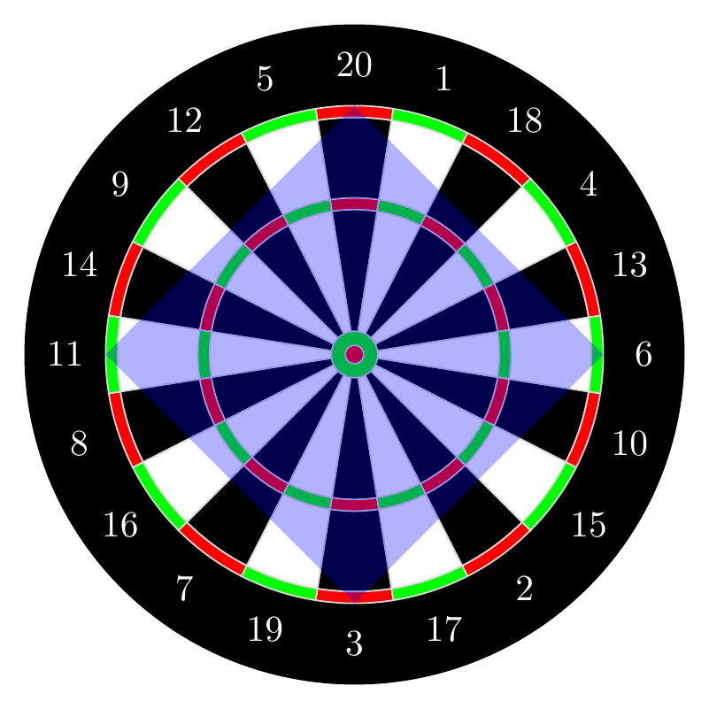
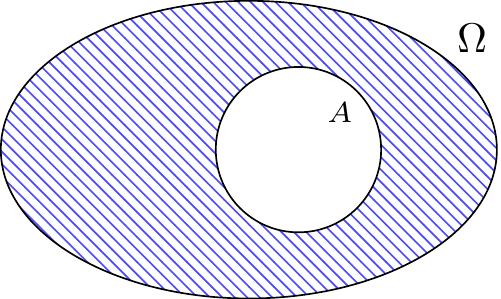
Example 3.2 (Throwing darts) A novice is throwing a dart at a dartboard, shown in Figure 3.1. Because the novice has poor aim, the dart is equally likely to land anywhere on the dartboard. What is the probability that the dart lands in the blue square shown?

Figure 3.1: Dartboard and a region of interest.

If the radius of the dartboard is $r$ inches, then:

the area of the dartboard is $\pi r^2$
the area of the blue square is $2 r^2$ (because its diagonal is the diameter of the dartboard, $2r$, so the side lengths are $r\sqrt{2}$)

Therefore, if the dart is equally likely to land anywhere on the dartboard, the probability must be \[ P(\text{dart lands in \textcolor{blue}{blue square}}) = \frac{2 r^2}{\pi r^2} = \frac{2}{\pi}. \tag{3.1}\]

But if we try to apply the classical definition of probability (Definition 1.3), there are infinitely many points where the dart could land, both on the dartboard and in the blue square, yielding the unhelpful answer \[ P(\text{dart lands in \textcolor{blue}{blue square}}) \overset{?}{=} \frac{|\{ \text{dart lands in \textcolor{blue}{blue square}} \}|}{|\Omega|} = \frac{\infty}{\infty} \]

In fact, the classical definition could never produce a probability of $\frac{2}{\pi}$ because the classical definition always results in a ratio of integers, whereas $\frac{2}{\pi}$ is an irrational number.

To handle situations like those in Example 3.1 and Example 3.2, we need a more general definition of probability. But before we present that definition, we examine more carefully why the classical definition of probability failed in those two examples.

The classical definition of probability broke down because there were infinitely many outcomes in the sample space. But it is not just that there were infinitely many—there are so many that we cannot even list them all. This is called an uncountable infinity.

Example 3.3 (Countable and uncountable infinities) An infinite set is called countable if it is possible to list the elements in a way that eventually covers every element.

For example, the set of integers $\mathbb{Z}$ is countable because we can list alternating positive and negative integers

$0$
$1$
$-1$
$2$
$-2$
and so on…

so that every integer eventually appears in this (infinite) list. It turns out that the set of rational numbers $\mathbb{Q}$ is also countable.

Now let us consider the sample space of all possible infinite sequences of coin flips from Example 3.1. Is this set also countable? Surprisingly, the answer is no! The argument, discovered by the mathematician Georg Cantor (1845-1918), starts by assuming that this set is countable and deriving a contradiction.

Assume, for the sake of contradiction, that it is possible to list all infinite sequences of coin flips. The list might look something like this:

HTHTHTHT...
HHHTTTHH...
TTTHTTTT...
TTHTHTHT...
HHTTHTHT...
THTTHTHT...
and so on…

We can construct a new sequence that is guaranteed to not be in this list, as follows.

Take the 1st flip from sequence 1 and change it. (For the list above, H $\to$ T.)
Take the 2nd flip from sequence 2 and change it. (For the list above, H $\to$ T.)
Take the 3rd flip from sequence 3 and change it. (For the list above, T $\to$ H.)
and so on…

Now, assemble a sequence out of the changed coin flips. For the hypothetical list above, this new sequence would be

TTHHTH...

This new sequence cannot possibly be in the list because it differs from the $i$th sequence in the $i$th position (and possibly in other positions as well). This is a contradiction because we assumed the list already contained all possible sequences, yet we just constructed a sequence that is not in the list. Therefore, the set of all possible infinite sequences of coin flips is not countable.

Sets that are not countable are called uncountable. Another example of an uncountable set is the real numbers $\mathbb{R}$. Because each outcome on a dartboard in Example 3.2 is a pair of coordinates $(x, y)$, each of which is a real number, the number of possible outcomes on a dartboard is also uncountable.

3.1 Set Theory Background

The key takeaway from the preceding discussion is that it is not always possible to define probability at the level of outcomes. Instead, we will define probability at the level of events.

Recall that an event is simply a set of outcomes. The “probability” $P(\cdot)$ is simply a function that assigns a number to each event in a “sensible” way. We will define what it means for $P$ to be “sensible” in Section 3.2, but in order to make sense of that definition, we will need some notation and terminology from set theory, the mathematical study of sets.

3.1.1 Intersections and Mutually Exclusive Events

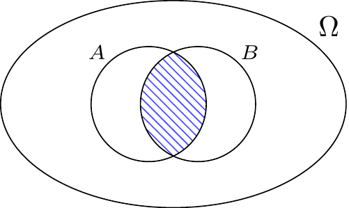
The intersection $A \cap B$ of two events $A$ and $B$, depicted in Figure 3.2, is the event that both $A$ and $B$ happen. Colloquially, we refer to $A \cap B$ as “$A$ and $B$.”

Figure 3.2: Two events $A$ and $B$ in a sample space $\Omega$ with their intersection $A \cap B$ marked in blue.

Example 3.4 (Bets on “red” and “even” in roulette) Consider a gambler who bets on both “red” and “even” on one spin of a roulette wheel (Figure 1.5). If $A$ is the event that she wins the “red” bet and $B$ is the event that she wins the “even” bet, then \[ A \cap B = \{ 12, 14, 16, 18, 30, 32, 34, 36 \} \] is the event that she wins both bets.

By counting the outcomes above, we see that \[ P(A \cap B) = \frac{8}{38}. \]

The intersection is an associative operation. When dealing with the intersection of more than two sets, the order in which the intersections are performed is irrelevant. Mathematically, \[ A \cap (B \cap C) = (A \cap B) \cap C. \] So we can write the above set as $A \cap B \cap C$ (omitting parentheses entirely) without any risk of confusion. This comes in handy in examples like the following.

Example 3.5 (Secret Santa and intersections) Recall Example 1.7, where four friends draw slips to decide who they will buy a gift for.

Let $E_i$ be the event that friend $i$ draws their own name. Then, \[ E_1 \cap E_2 \cap E_3 \cap E_4 \] represents the event that everyone draws their own name. A shorthand for the above event is \[ \bigcap_{i=1}^4 E_i. \]

By counting the outcomes in the sample space of Example 1.7, we see that \[ P\left(\bigcap_{i=1}^4 E_i\right) = \frac{1}{24}. \]

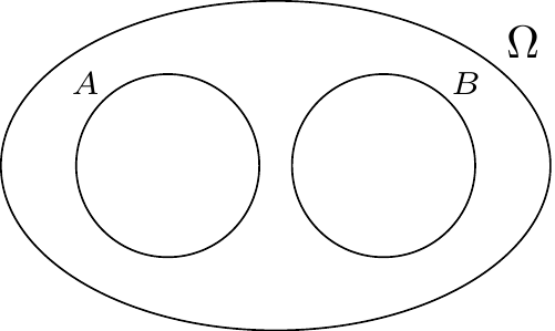
We refer to a collection of events as disjoint when their intersection is empty (i.e., they share no outcomes). Disjoint events are also referred to as mutually exclusive because no two of them can happen simultaneously. Figure 3.3 depicts two disjoint events.

Figure 3.3: Two mutually exclusive events $A$ and $B$ in a sample space $\Omega$.

Disjoint sets play a critical role in the rigorous definition of probability, as we will see in Section 3.2. For now, we give some examples of disjoint (or mutually exclusive) events.

Example 3.6 (Mutually exclusive events) In roulette, if $A$ is the event that the ball lands in a red pocket and $B$ is the event that the ball lands in a black pocket on a single spin of the roulette wheel, then \[ A \cap B = \{ \}, \] since each pocket is either red or black, not both.

Here is a more subtle example. In Secret Santa (Example 3.5), the event \[ E_1 \cap E_2 \cap E_3 \] that the first three friends draw their own name is disjoint from the event \[ E_4^c, \] which denotes the event that $E_4$ does not happen (called the complement of $E_4$, which we discuss further in Section 3.1.3), that the fourth friend does not draw their own name. To see this, observe that if the first three friends all draw their own names, then there is only one slip for the fourth friend, which is necessarily their own slip. Therefore, $E_4$ must happen if $E_1 \cap E_2 \cap E_3$ does.

Another way to see this is to list the outcomes in each set: \[ \begin{align} (E_1 \cap E_2 \cap E_3) \cap E_4^c &= \{ 1234 \} \cap \{ 1243, 1342, \dots, 4321 \} \\ &= \{ \}. \end{align} \]

3.1.2 Unions and Disjoint Unions

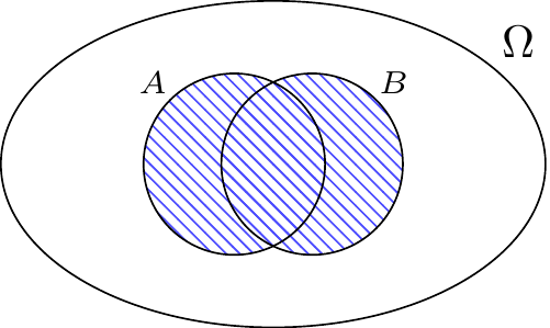
The union $A \cup B$ of two events $A$ and $B$, depicted in Figure 3.4, is the event either $A$ happens or $B$ happens (or both happen). Colloquially, we refer to $A \cup B$ as “$A$ or $B$.”

Figure 3.4: Two events $A$ and $B$ in a sample space $\Omega$ with their union $A \cup B$ marked in blue.

Example 3.7 (Winning at least one bet in roulette) Recall from Example 3.4 the gambler who bets on both “red” and “even” on one spin of a roulette wheel. If $A$ is the event that she wins the “red” bet and $B$ is the event that she wins the “even” bet, then \[ A \cup B \] is the event that she wins at least one bet.

We can count the outcomes in $A \cup B$ to obtain \[ P(A \cup B) = \frac{28}{38}. \]

Like the intersection, the union is also an associative operation. When dealing with the union of more than two sets, the order in which the intersections are performed is irrelevant. Mathematically, \[ A \cup (B \cup C) = (A \cup B) \cup C. \] So we can write the above set as $A \cup B \cup C$ (omitting parentheses entirely) without any risk of confusion. This comes in handy in examples such as the following.

Example 3.8 (Secret Santa and unions) Let $E_i$ be the event that the $i$th friend draws their own name, as in Example 3.5. Then, the event \[ E_1 \cup E_2 \cup E_3 \cup E_4 \] is the unfortunate event that someone (i.e., at least one person) draws their own name. A shorthand for the above event is \[ \bigcup_{i=1}^4 E_i. \]

By counting the outcomes in the sample space of Example 1.7, we see that \[ P\left(\bigcup_{i=1}^4 E_i\right) = \frac{15}{24}. \]

The union of disjoint (or mutually exclusive) events is called a disjoint union.

3.1.3 Complements

The complement $A^c$ of an event $A$, depicted in Figure 4.2, is the event that $A$ does not happen. Colloquially, we refer to $A^c$ as “not $A$”.

Figure 3.5: An event $A$ in a sample space $\Omega$ with its complement $A^c$ marked in blue.

We already encountered the complement in Example 3.6, where we saw that $E_4^c$ is the event that the fourth friend does not drawn their own name.

Here are some identities that are useful for simplifying the complement of a complex event involving intersections and unions.

Theorem 3.1 (De Morgan’s Laws) Let $A$ and $B$ be events. Then,

\[ \begin{align*} (A \cup B)^c &= A^c \cap B^c \\ (A \cap B)^c &= A^c \cup B^c \end{align*} \tag{3.2}\]

De Morgan’s Laws simply say that when taking the complement of a complex event, we take the complement of each individual event in the complex event and convert $\cup$ to $\cap$ (and vice versa). The next example demonstrates how De Morgan’s Laws can be used to determine the complement.

Example 3.9 (Complement of no one drawing their own name in Secret Santa) In the notation of Example 3.5, the event that no one draws their own name is \[ E_1^c \cap E_2^c \cap E_3^c \cap E_4^c. \]

What is the complement of this event? A common misconception is that the complement is that everyone draws their own name. De Morgan’s Laws come in handy whenever there is any doubt. \[ (E_1^c \cap E_2^c \cap E_3^c \cap E_4^c)^c = E_1 \cup E_2 \cup E_3 \cup E_4. \]

In other words, the complement of “no one draws their own name” is “at least one person draws their own name,” an event which we already studied in Example 3.8.

3.2 The Axioms of Probability

In 1933, mathematician Andrey Kolmogorov used set theory to establish the modern axiomatic foundation of probability, which remains the standard rigorous framework used today. In Kolmogorov’s formulation, probabilities are determined by a probability function $P$. This function assigns a probability $P(A)$ between $0$ and $1$ to each event $A$ in the sample space. To be a valid probability function, $P$ must satisfy the three Kolmogorov axioms, which we present below.

Figure 3.6: Andrey Kolmogorov (1903-1987)

Definition 3.1 (Axiomatic definition of probability) Consider a sample space $\Omega$ and function $P$ that maps events $A \subseteq \Omega$ to real numbers. We say that $P$ is a probability function if it satisfies the following three axioms:

Non-negativity: Probabilities are never negative: $P(A) \geq 0$.
Normalization: The probability of the entire sample space is one and the probability of the empty set is zero; i.e.,

\[ P(\Omega) = 1 \quad. \]

Countable additivity: If $A_1, A_2, A_3, …$ are a countable collection (defined in Example 3.3) of disjoint sets (mutually exclusive events), then

\[ P\left( \bigcup_{i=1}^{\infty} A_i \right) = \sum_{i=1}^{\infty} P(A_i). \]

Here are some properties that follow from the axioms. Sometimes these properties are taken to be part of the axioms, but there is no reason to treat these as axioms, since they can be proven.

Proposition 3.1 (Immediate consequences of the axioms) If we let $A_1, A_2, \dots$ all be the empty set $\{ \}$, then they constitute a disjoint collection whose union is also the empty set $\{ \}$. Therefore, by countable additivity (Axiom 3), \[ P(\{ \}) = \sum_{i=1}^\infty P(\{ \}). \] In other words, the probability of the empty set is a number which, when added to itself infinitely many times, is itself. The only number with this property is zero, so \[ P(\{ \}) = 0. \tag{3.3}\]

Furthermore, countable additivity is a stronger assumption than we need for most problems. In everyday probability questions, there are usually only finitely many disjoint events $A_1, \dots, A_n$. Fortunately, finite additivity \[ P\left(\bigcup_{i=1}^n A_i\right) = \sum_{i=1}^n P(A_i) \tag{3.4}\] follows directly from countable additivity, as we ask you to show in Exercise 3.2.

Should Axiom 3 be replaced by finite additivity?

Some thinkers, most notably Bruno de Finetti (whom we will encounter in Section 3.3), have argued that countable additivity is too strong of an assumption, and Axiom 3 should be replaced by finite additivity (Equation 3.4). This seemingly innocuous change breaks many important results in probability theory, so we do not explore that possibility in this book.

Unlike the classical definition of probability, which provides a prescription for calculating probabilities, Kolmogorov’s axiomatic definition only offers properties that a probability function $P$ must satisfy. There are many possible functions that satisfy these axioms, as the next example illustrates.

Example 3.10 (Rolling a loaded die) A die has six possible outcomes: \[ \Omega = \{ 1, 2, 3, 4, 5, 6 \}. \]

Previously, we assumed the die was fair, so the probability function satisfied \[ P(A) = \frac{|A|}{|\Omega|}. \] In particular, this implies that the probability of each outcome is the same: \[ \begin{align} P(\{ 1\}) &= P(\{ 2 \}) = P(\{ 3\}) = P(\{ 4 \}) = P(\{ 5\}) = P(\{ 6 \}) = \frac{1}{6}. \end{align} \]

However, nothing in Definition 3.1 requires that we use this probability function. For example, the gambler could have cheated by loading the die so that sixes come up more often. In that case, the probabilities might instead be \[\begin{align*} & P(\{1\}) = 0.10, \ \ P(\{2\}) = 0.15 , \ \ P(\{3\}) = 0.15, \\ & P(\{4\}) = 0.15, \ \ P(\{5\}) = 0.15, \ \ P(\{6\}) = 0.30. \end{align*}\] What about the probabilities of other events in this sample space? In fact, all of the remaining probabilities are already determined by Axiom 3. To see why, consider the probability of rolling an even number. We can write it as a disjoint union of the outcomes in the set: \[ \begin{align*} P(\{ 2, 4, 6 \}) &= P(\{2\} \cup \{4\} \cup \{6\}) \\ &= P(\{2\}) + P(\{4\}) + P(\{6\}) & \text{(Axiom 3)} \\ &= 0.15 + 0.15 + 0.30 & \text{(choice of } P \text{)} \\ &= 0.60. \end{align*} \]

Similar reasoning allows us to compute the probability of any event under $P$.

Example 3.10 demonstrates that Kolmogorov’s axiomatic definition is a generalization of the classical definition. The classical definition is only able to describe fair dice, but the axiomatic definition is also able to describe loaded dice.

As promised, the flexibility of Kolmogorov’s definition allows us to handle the problematic examples from the beginning of this chapter.

Example 3.11 (Infinite tosses of a fair coin, axiomatic version) Recall the sample space from Example 3.1, which consisted of all infinite sequences of heads and tails. The axiomatic definition of probability attempts to assign a probability to any set of sequences.

For example, let \[ A_i \overset{\text{def}}{=}\{ \omega: \text{$\omega_i$ is heads} \}. \] Then, examples of sequences in $A_2$ include:

THTHHHH...
HHHHTTH...
THHTTTT...
HHTHHHT...
and so on…

In other words, $A_2$ consists of all sequences with an H in the second position.

Now, we can write many events of interest in terms of $A_1, A_2, \dots$, and define their probabilities accordingly. For example,

The probability that the second toss is heads is $P(A_2) = \frac{1}{2}$.
The probability that heads first appears on the second toss is $P(A_1^c \cap A_2) = \frac{1}{4}$.
The probability that the first three tosses are all heads is $P(A_1 \cap A_2 \cap A_3) = \frac{1}{8}$.
More generally, a event that specifies that any $k$ tosses are heads has probability \[ P(A_{i_1} \cap A_{i_2} \cap \dots \cap A_{i_k}) = \frac{1}{2^k}. \tag{3.5}\] Because a coin is just as likely to land tails as heads, the probability remains the same if we replace any $A_{i_j}$ in the event above by its complement $A_{i_j}^c$.

A surprising variety of events can be expressed in terms of $A_1, A_2, \dots$, as Exercise 3.4 asks you to show. For such events, the axioms can be used in conjunction with Equation 3.5 to calculate their probabilities.

However, not all events can be easily expressed in terms of $A_1, A_2, \dots$. For example, based on the frequentist interpretation of probability, we might expect the frequency of heads to be “close” to $1/2$ after a large number of tosses. That is, for any $\epsilon > 0$, we might expect \[ P\left(\Big|\frac{\text{number of heads after $n$ tosses}}{n} - \frac{1}{2}\Big| < \epsilon\right) \] to be close to $1$ as $n$ increases. It is not straightforward to determine the probability of events like these. Nevertheless, the axiomatic definition requires that $P$ assign a probability even to sets like these.

Events that cannot be assigned a probability

In fact, there are so many possible sets that there are even sets that cannot be assigned a reasonable probability. These sets are called non-measurable sets. A construction of a non-measurable set is described in Exercise 3.5. However, be warned: non-measurable sets are mathematical curiosities for the most part; they do not correspond to natural events in the real world. As such, they can be ignored in applications of probability to practical problems.

Example 3.12 (Throwing darts, axiomatic version) Recall Example 3.2, where a novice was throwing a dart so that the dart was equally likely to land anywhere on the dartboard.

The probability function $P$ assigns a probability to each region of the dartboard. For example, we argued that the probability of the blue square in Figure 3.1 should be \[ P(\text{dart lands in \textcolor{blue}{blue square}}) = \frac{\text{area of \textcolor{blue}{blue square}}}{\text{area of dartboard}} = \frac{2}{\pi}. \] In general, the probability of any region $A$ should be proportional to the area of $A$: \[ P(\text{dart lands in $A$}) = \frac{\text{area of $A$}}{\text{area of dartboard}}. \tag{3.6}\]

We can check that the probability function defined by Equation 3.6 satisfies the axioms of probability:

Areas cannot be negative, so $P(A) \geq 0$.
The probability of the sample space (i.e., the dartboard) is \[ P(\Omega) = \frac{\text{area of dartboard}}{\text{area of dartboard}} = 1. \]
If regions $A_1, A_2, \dots$ are disjoint, then they do not overlap. The area of their union $A_1 \cup A_2 \cup \dots$ can be calculated by simply adding up the individual areas.

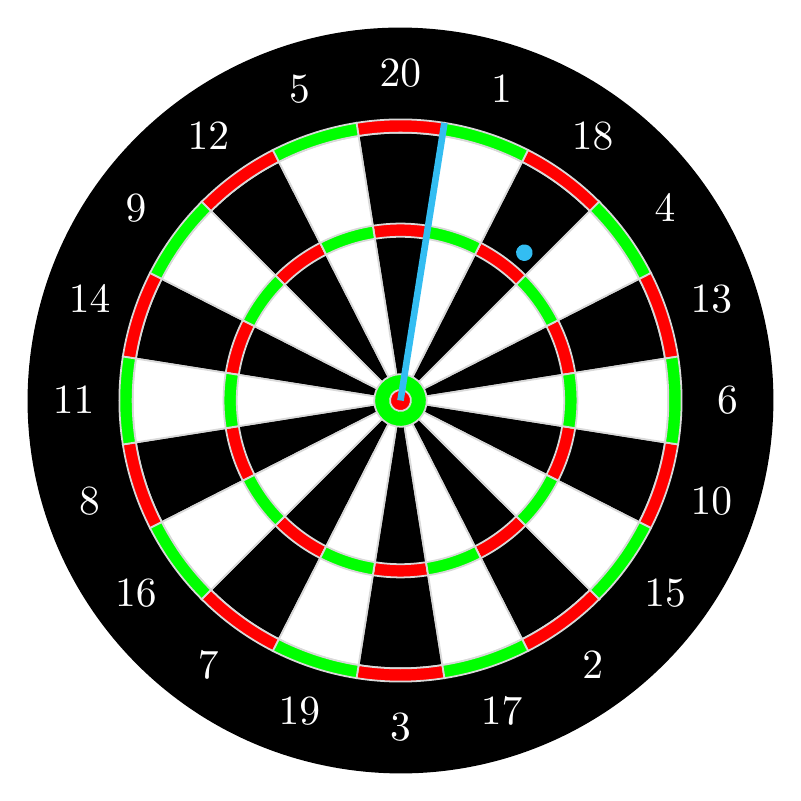
Figure 3.7: Any point or line on a dartboard has probability zero.

One consequence of Equation 3.6 is that many events have probability zero. Two such events are depicted in cyan in Figure 3.7.

The probability that the dart hits any particular point on the dartboard is $0$ because a point has no area.
The probability that the dart lands on any particular line on the dartboard, such as the boundary between the 20 and 1 sectors, is also $0$ because a line is infinitely thin and has no area.

Phrased another way: the probability that the dart hits the dartboard is $1$, but the probability that the dart hits any point on the dartboard is $0$. Exercise 3.6 invites you to ponder this paradox further.

Thus, Kolmogorov’s axiomatic framework lets us rigorously assign probabilities to both finite and infinite sample spaces. It successfully resolves the issues raised in Example 3.1 and Example 3.2.

3.3 Interpretations of Probability

There are two principal ways people interpret probabilities: the frequentist approach and the subjectivist approach. We initially introduced the frequentist viewpoint in Chapter 1, but as we will see, it has limitations.

The frequentist viewpoint assumes that the experiment can be repeated infinitely under identical conditions. But in reality, repeated expriments almost always occur under slightly changing conditions, making the strict frequentist notion of “identical conditions” difficult to satisfy. For example, the election forecaster FiveThirtyEight gave Donald Trump a $.286$ probability of winning the 2016 U.S. presidential election. However, the 2016 presidential election only happened once. Although Trump ran again in 2020 and 2024, these were different voters under different circumstances. What would it mean to infinitely repeat the 2016 presidential election?

It is not even clear that a roulette wheel can be spun repeatedly under identical conditions. A roulette wheel will be worn down by repeated spins, and each time it is spun, the molecules in the surrounding air will have a different configuration.

Because of these objections to the frequentist interpretation, the Italian statistician Bruno de Finetti (1906-1985) developed the subjective interpretation of probability. In this view, $P(A)$ simply represents an individual’s personal degree of belief about the occurrence of $A$. Unlike the frequentist interpretation, the subjective interpretation does not rely on repeated trials. For instance, to assert that Trump had a $.286$ probability of winning the 2016 election only reflects the judgment of a particular forecaster.

One way to make “beliefs” concrete is to relate them to betting. Specifically, if an individual believes that the probability of $A$ is $P(A)$, then they should be willing to engage in any bet where they pay or receive $\$1$ if $A$ occurs, for a price of $\$P(A)$. For example, FiveThirtyEight should have been willing to stake $\$0.286$ for a possible payout of $\$1$ if Trump won the 2016 election, and they should equally have agreed to take $\$0.286$ from anyone in exchange for paying them $\$1$ if Trump won the election.

Where do Kolmogorov’s axioms fit into the subjective interpretation of probability? They codify necessary conditions for an individual’s beliefs to be rational or coherent. If an individual’s beliefs do not satisfy Kolmogorov’s axioms, then it is possible to get them to agree to a series of bets which guarantees that you make a profit from them. Such a series of bets is called a Dutch book; economists would call this arbitrage.

For example, consider an individual whose beliefs violate Axiom 1 (non-negativity). That is, there is an event $A$ for which she believes $P(A) < 0$. This means that she would be willing to accept a negative price for a bet; that is, she would pay you to take the bet. If $A$ occurs, then she pays you an additional $\$1$; otherwise, she does not pay any additional money, but she has already paid you to take the bet. No matter what happens, she loses money, so this is an arbitrage opportunity.

What if an individual’s beliefs violate Axiom 2 (normalization)? To be specific, suppose he believes that $P(\Omega) < 1$. Then, he would be willing to take a bet for $\$P(\Omega)$ that pays out $\$1$ when $\Omega$ happens. But $\Omega$ is the entire sample space, so he will always pay out $\$1$, for a net loss of $\$1 - P(\Omega)$. A similar argument can be used to exploit someone who believes $P(\Omega) > 1$; the details are requested in Exercise 3.8.

It is less obvious why Axiom 3 (additivity) is necessary for beliefs to be rational. In the next example, we construct a Dutch book for a person whose beliefs violate additivity.

Example 3.13 (Necessity of additivity for the subjectivist) Consider the following mutually exclusive events, based on the point spread of a football game between the Philadelphia Eagles and the Dallas Cowboys:

$A$: Eagles win by at least 5 points.
$B$: Cowboys win by at least 5 points.
$A \cup B$: The point spread is at least 5.

Suppose that Pat believes \[ P(A \cup B) = 0.70 \] but \[ \begin{align} P(A) &= 0.40 & P(B) &= 0.20, \end{align} \] violating additivity (Axiom 3). How could we arbitrage Pat’s beliefs?

Based on his beliefs, Pat should be willing to accept the following bets:

Wager $\$0.70$ for a bet that pays $\$1$ if the point spread is at least 5.
Take $\$0.40$ for a bet that pays $\$1$ if the Eagles win by at least 5 points.
Take $\$0.20$ for a bet that pays $\$1$ if the Cowboys win by at least 5 points.

Note that Pat is already down after these initial wagers: \[ -\$0.70 + \$0.40 + \$0.20 = -\$0.10. \]

Now, this bet could resolve in one of three mutually exclusive ways:

$A$ (Eagles win by at least 5): Pat receives $\$1$ from the first bet and pays out $\$1$ from the second bet.
$B$ (Cowboys win by at least 5): Pat receives $\$1$ from the first bet and pays out $\$1$ from the third bet.
$(A \cup B)^c$ (Point spread is less than 5): Pat receives nothing from all three bets.

No matter what happens, Pat’s net loss is $\$0.10$ (from the initial wagers). Therefore, we have successfully arbitraged his irrational beliefs.

There is nothing special about these particular probabilities or the Eagles-Cowboys game. The same argument can be used to arbitrage someone who believes that \[ P(A \cup B) > P(A) + P(B) \] for any disjoint events $A$ and $B$. Exercise 3.9 asks you to complete the proof.

Although the subjective interpretation of probability may feel like an abstract philosophical concept, it has at least one significant practical application: prediction markets. Prediction markets invite bettors to bet money on various world events. Based on how much people are willing to bet, they can estimate the probability of those events.

In summary, Kolmogorov’s axioms serve as a universal mathematical framework that underlies both frequentist and subjectivist interpretations. Whether we view probability as the limit of relative frequencies or as degrees of belief, the axioms ensure internal consistency and avoid Dutch book scenarios.

3.4 Exercises

Exercise 3.1 (Poker and set theory) [*]

You are dealt a five-card hand from a shuffled deck of cards. Let $A_i$ be the event that card $i$ is a heart, where $i=1, 2, 3, 4, 5$.

Match each description of the event in symbols (set theory notation) to the description of the event in words (plain English). Which events are complements of one another?

Event (in symbols)	Event (in words)
1. $\displaystyle \bigcup_{i=1}^5 A_i$	A. flush of hearts
2. $\displaystyle \bigcap_{i=1}^5 A_i$	B. at least one heart
3. $\displaystyle \bigcup_{i=1}^5 A_i^c$	C. at least one card is not a heart
4. $\displaystyle \bigcap_{i=1}^5 A_i^c$	D. no hearts

Exercise 3.2 (Finite additivity) [**]

Prove that Kolmogorov’s axioms (Definition 3.1) imply finite additivity. That is, if $A_1, A_2, \dots, A_n$ are a disjoint events, then \[ P\left(\bigcup_{i=1}^n A_i \right) = \sum_{i=1}^n P(A_i). \]

Hint: What happens if you let $A_{n+1} = A_{n+2} = \dots = \{ \}$?

Exercise 3.3 (Uniform probability function) [**]

Let the sample space $\Omega = \{ 1, 2, 3, \dots \}$ be the set of natural numbers. Show that it is impossible to have a probability function $P$ that assigns equal probability to each individual outcome.

Remark: Note that countable additivity is necessary to derive a contradition. If Axiom 3 were replaced by finite additivity, then it would be possible to define a probability function $P$ that assigns equal probability to each outcome.

Exercise 3.4 (Intersections and unions of infinitely many events) [***]

Let $\Omega$ be the sample space of all infinite sequences of coin tosses, as in Example 3.11. Let $A_i$ be the event that the $i$th toss is heads, where $i=1, 2, 3, \dots$.

Describe each of the following events in plain English, and determine the complement of each event (in symbols and in plain English).

$\displaystyle \bigcap_{i=1}^\infty A_i$
$\displaystyle \bigcup_{i=1}^\infty A_i$
$\displaystyle \bigcap_{n=1}^\infty \bigcup_{i=n}^\infty A_i$
$\displaystyle \bigcup_{n=1}^\infty \bigcap_{i=n}^\infty A_i$

Exercise 3.5 (An event that cannot be assigned a probability) [****]

Consider the sample space of Example 3.1, where we toss a fair coin infinitely many times. Here is an event that cannot be assigned a probability in a sensible way. (Admittedly, this event is a bit contrived and difficult to interpret.)

Suppose we call two sequences of coin flips “equivalent” if the sequences are identical eventually. For example, the following sequences start differently, but they all eventually end in ...HTHTH... (alternating heads and tails on the even and odd tosses):

HTTHTHTHTH...
THTHTHTHTH...
HHHTTHTHTH...

Now, define an event $A$ as follows: from each set of “equivalent” sequences, choose one (and only one) “representative” sequence. So for example, one element of $A$ might be the sequence THTHTHTHTH... above. But if this sequence is in $A$, then the other two sequences above are definitely not in $A$.

Show that there is no sensible way to assign a probability to $A$ satisfying the axioms of probability.

Hint:

Define transformations of a sequence $\omega$ of coin flips as follows. For any finite set $I$ of indices, $t_I(\omega)$ flips the result of the $i$th toss for all $i \in I$, so if the $i$th toss is H, it becomes T, and vice versa. For example, $t_{\{1, 3, 4 \}}($THTHTHTHTH...$)=$ HHHTTHTHTH....

What can you say about $P(t_I(A))$?
Argue that $\bigcup_I t_I(A)$ is a disjoint countable union. What is the union?
Derive a contradiction with the probability axioms.

Exercise 3.6 (A dartboard paradox) [**]

Where is the flaw in the following argument?

The dartboard $\Omega$ can be written as a union of all of the points on the dartboard. \[ \Omega = \bigcup_{(x, y) \in \Omega} \{ (x, y) \}. \] Each point is, of course, disjoint from any other point. By Axiom 3, \[ P(\Omega) = \sum_{(x, y) \in \Omega} P(\{ (x, y) \}). \] But the left-hand side is equal to $1$ (by Axiom 2), while the right-hand side is equal to $0$ (since the probability of any individual point on the dartboard is $0$).

Therefore, $1 = 0$.

Exercise 3.7 (Weather forecasting) [*]

Weatherman Phil Connors believes the following about the weather tomorrow (Groundhog Day, of course):

$P(\{ \text{rain}, \text{shine} \}) = 0.8$
$P(\{ \text{rain}, \text{snow} \}) = 0.1$
$P(\{ \text{shine}, \text{snow} \}) = 0.5$

Do his beliefs violate the axioms of probability? Justify your answer using the axioms carefully.

Exercise 3.8 (Necessity of Axiom 2 for the subjectivist) [**]

In Section 3.3, we showed that an individual who believes that $P(\Omega) < 1$ can be arbitraged. Construct a series of bets (i.e., a “Dutch book”) to arbitrage an individual who believes that $P(\Omega) > 1$, thereby showing that Axiom 2 ($P(\Omega) = 1$) is necessary.

Exercise 3.9 (Necessity of Axiom 3 for the subjectivist) [**]

Show how a person can be arbitraged if their beliefs are not consistent with Axiom 3. That is, they believe that there are disjoint events $A$ and $B$ for which \[ P(A \cup B) \neq P(A) + P(B). \]

Hint: Set up separate Dutch books for the two cases:

$P(A \cup B) > P(A) + P(B)$
$P(A \cup B) < P(A) + P(B)$