A child is born to parents who are carriers for the recessive alleles of two genes. That is, both parents have genetic makeup \(AaBb\). Let \(X\) be the number of copies of the dominant \(A\) allele that the child inherits and \(Y\) be the number of copies of the dominant \(B\) allele.
Since the child independently has a \(1/2\) chance of inheriting an \(A\) allele from each parent, the total number of copies of \(A\) they inherit is \(X \sim \text{Binomial}(n=2, p=1/2)\). By the same reasoning for the \(B\) allele, \(Y \sim \text{Binomial}(n=2, p=1/2)\).
However, this tells us nothing about the relationship between \(X\) and \(Y\). In this chapter, we will develop tools to describe the relationship between two random variables. As we will see, even with the information given above, the relationship between \(X\) and \(Y\) can vary widely.
Joint PMF
One way to describe the relationship between two random variables is by the joint PMF, which specifies the probability of every possible combination of values \((x,y)\).
Definition 13.1 (Joint PMF of \(X\) and \(Y\)) The joint distribution of two random variables \(X\) and \(Y\) is described by the joint PMF \[
f_{X,Y}(x,y) \overset{\text{def}}{=}P(X = x, Y = y).
\tag{13.1}\]
First, we consider the joint PMF of two random variables that have “no relationship”. The notion of independence from Chapter 6 is one way to formalize what it means for two random quantities to have “no relationship”. The following definition is motivated by the definition of independent events (Proposition 6.1).
Definition 13.2 (Independent Random Variables) Two (discrete) random variables \(X\) and \(Y\) are independent if \[
P(X = x, Y = y) = P(X = x) P(Y = y)
\tag{13.2}\] for all values \(x\) and \(y\).
We can restate Equation 13.2 in terms of the joint PMF and the PMFs of \(X\) and \(Y\) individually: \[
f_{X, Y}(x,y) = f_X(x) f_Y(y)
\tag{13.3}\] for all values \(x\) and \(y\).
Returning to the genetics example from the beginning of this chapter, \(X\) and \(Y\) are independent if the two genes are on different chromosomes.
Example 13.1 (Joint PMF under independent assortment) If \(X\) and \(Y\) represent the numbers of dominant alleles for two genes on different chromosomes, then Mendel’s Law of Independent Assortment (Example 6.3) applies, and their joint PMF can be obtained by multiplying their individual PMFs, which we know to be \(\text{Binomial}(n=2, p=1/2)\).
\[
\begin{align}
f_{X,Y}(x,y) &= f_{X}(x) f_Y(y) \\
&= \binom{2}{x} \left( \frac{1}{2} \right)^x \left( \frac{1}{2} \right)^{2-x} \cdot \binom{2}{y} \left( \frac{1}{2} \right)^y \left( \frac{1}{2} \right)^{2-y} \\
&= \binom{2}{x} \binom{2}{y} \left( \frac{1}{2} \right)^{4},
\end{align}
\]
where \(x, y = 0, 1, 2\). It is customary to arrange these probabilities in a table, as follows.
| \(0\) \((bb)\) |
\(0.0625\) |
\(0.125\) |
\(0.0625\) |
| \(1\) \((Bb)\) |
\(0.125\) |
\(0.25\) |
\(0.125\) |
| \(2\) \((BB)\) |
\(0.0625\) |
\(0.125\) |
\(0.0625\) |
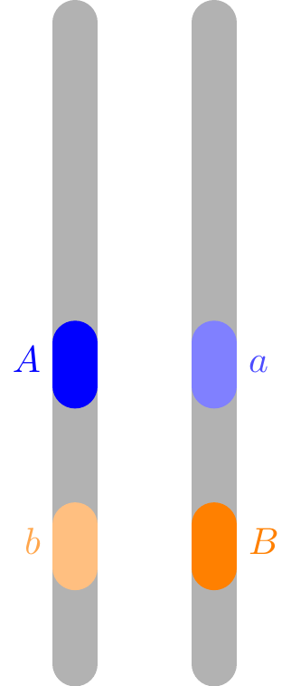
However, it is common for two genes to deviate from the joint distribution predicted by Example 13.1. This is because \(X\) and \(Y\) are no longer independent if the two genes are on the same chromosome. Figure 13.1 illustrates a possible configuration of two genes for a carrier with genetic makeup \(AaBb\). In this example, the \(A\) allele is on the same chromosome as the \(b\) allele. Therefore, the parent will pass down the \(A\) and \(b\) alleles together or the \(a\) and \(B\) alleles together. The two genes are no longer inherited independently. This phenomenon, where genes tend to be inherited together, is called linkage.
Example 13.2 (Joint PMF with linkage) If both parents have the pair of chromosomes shown in Figure 13.1 and independently pass one of them down, then there are four equally likely possibilities for the genes inherited by the child: \((Ab, Ab)\), \((Ab, aB)\), \((aB, Ab)\), and \((aB, aB)\). Counting the \(A\)s and \(B\)s in each case, we obtain the following probabilities:
- \(P(X = 2, Y = 0) = \frac{1}{4}\)
- \(P(X = 1, Y = 1) = \frac{2}{4}\)
- \(P(X = 0, Y = 2) = \frac{1}{4}\).
In other words, \(Y = 2 - X\), and the joint PMF table looks as follows.
| \(0\) |
\(0\) |
\(0\) |
\(0.25\) |
| \(1\) |
\(0\) |
\(0.5\) |
\(0\) |
| \(2\) |
\(0.25\) |
\(0\) |
\(0\) |
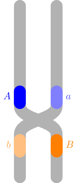
However, what usually happens when two genes are on the same chromosome is something between Example 13.1 and Example 13.2. There is a chance that the pair of chromosomes in Figure 13.1 could “recombine”, as shown in Figure 13.2, so that \(A\) is now on the same chromosome as \(B\) (and \(a\) is with \(b\)). One of these recombinant chromosomes is randomly passed down to the child.
Example 13.3 (Joint PMF with recombination) Suppose that both parents initially have the pair of chromosomes shown in Figure 13.1, and they each independently undergo recombination with probability \(0.1\) (which results in the configuration shown in Figure 13.2).
Deriving the joint PMF of \(X\) and \(Y\) is quite involved, but we calculate \(f_{X, Y}(1, 0)\) as an illustration of how this probability is no longer zero under recombination. We use the Law of Total Probability (Theorem 7.1), conditioning on whether \(0\), \(1\), or \(2\) parents undergo recombination. \[
\begin{align}
f_{X, Y}(1, 0) = P(X = 1, Y = 0) &= \phantom{.} P(\text{no recombination}) \cdot P(X = 1, Y = 0 \mid \text{no recombination}) \\
&\quad + P(\text{1 recombination})\cdot P(X = 1, Y = 0 \mid \text{1 recombination}) \\
&\quad + P(\text{2 recombinations})\cdot P(X = 1, Y = 0 \mid \text{2 recombinations}) \\
&= \phantom{.} (0.9)^2 \cdot P(X = 1, Y = 0 \mid \text{no recombination}) \\
&\quad + 2(0.1)(0.9) \cdot P(X = 1, Y = 0 \mid \text{1 recombination}) \\
&\quad + (0.1)^2 \cdot P(X = 1, Y = 0 \mid \text{2 recombinations})
\end{align}
\]
As shown in Example 13.2, it is impossible for \(X = 1\) and \(Y = 0\) in the absence of recombination, so \[ P(X = 1, Y = 0 \mid \text{no recombination}) = 0. \] As for the other terms,
- If exactly one parent undergoes recombination, then that parent will pass down \(AB\) or \(ab\), while the other passes down \(Ab\) or \(aB\). Therefore, the child is equally likely to inherit one of the following: \((AB, Ab)\), \((AB, aB)\), \((ab, Ab)\), and \((ab, aB)\). Only one of these possibilities corresponds to \(X = 1\) and \(Y = 0\), so \[
P(X = 1, Y = 0 \mid \text{1 recombination}) = \frac{1}{4}.
\]
- If both parents undergo recombination, then both parents pass down either \(AB\) or \(ab\), in which case the number of \(A\) alleles always matches the number of \(B\) alleles (\(X = Y\)). Therefore, it is impossible for \(X = 1\) and \(Y = 0\): \[
P(X = 1, Y = 0 \mid \text{2 recombinations}) = 0.
\]
Therefore, \[
f_{X, Y}(1, 0) = 2(0.1)(0.9) \cdot \frac{1}{4} = 0.045.
\]
We can do the same for all possible values \(x, y = 0, 1, 2\).
Using the Law of Total Probability, \[
\begin{align}
P(X = x, Y = y) &= \phantom{.} (0.9)^2 \cdot P(X = x, Y = y \mid \text{0 recombinations}) \\
&\quad + 2(0.1)(0.9) \cdot P(X=x, Y=y \mid \text{1 recombination}) \\
&\quad + (0.1)^2 \cdot P(X = x, Y = y \mid \text{2 recombinations}).
\end{align}
\]
Notice that the joint PMF without recombination, \(P(X = x, Y = y \mid \text{no recombination})\), was already calculated in Example 13.2, so we just need to determine the other conditional probabilities.
- If exactly one parent undergoes recombination, then that parent will pass down \(AB\) or \(ab\), while the other passes down \(Ab\) or \(aB\). Therefore, there are four equally likely possibilities: \((AB, Ab)\), \((AB, aB)\), \((ab, Ab)\), and \((ab, aB)\). Counting the \(A\)s and \(B\)s in each case, we obtain
- \(P(X = 2, Y = 1 \mid \text{1 recombination}) = \frac{1}{4}\),
- \(P(X = 1, Y = 2 \mid \text{1 recombination}) = \frac{1}{4}\),
- \(P(X = 1, Y = 0 \mid \text{1 recombination}) = \frac{1}{4}\),
- \(P(X = 0, Y = 1 \mid \text{1 recombination}) = \frac{1}{4}\).
- If both parents undergo recombination, then both parents pass down either \(AB\) or \(ab\). Counting the \(A\)s and \(B\)s in each case, we obtain
- \(P(X = 2, Y = 2 \mid \text{2 recombinations}) = \frac{1}{4}\),
- \(P(X = 1, Y = 1 \mid \text{2 recombinations}) = \frac{2}{4}\),
- \(P(X = 0, Y = 0 \mid \text{2 recombinations}) = \frac{1}{4}\).
Now, we can combine all the probabilities to obtain the following table:
| \(0\) |
\((0.1)^2 \cdot \frac{1}{4}\) |
\(2(0.1)(0.9) \cdot \frac{1}{4}\) |
\((0.9)^2 \cdot \frac{1}{4}\) |
| \(1\) |
\(2(0.1)(0.9) \cdot \frac{1}{4}\) |
\((0.9)^2 \cdot \frac{2}{4} + (0.1)^2 \cdot \frac{2}{4}\) |
\(2(0.1)(0.9) \cdot \frac{1}{4}\) |
| \(2\) |
\((0.9)^2 \cdot \frac{1}{4}\) |
\(2(0.1)(0.9) \cdot \frac{1}{4}\) |
\((0.1)^2 \cdot \frac{1}{4}\) |
In the end, we obtain the following joint PMF.
| \(0\) |
\(0.0025\) |
\(0.045\) |
\(0.2025\) |
| \(1\) |
\(0.045\) |
\(0.41\) |
\(0.045\) |
| \(2\) |
\(0.2025\) |
\(0.045\) |
\(0.0025\) |
As a sanity check, we can make sure that the probabilities in this table add up to \(1\).
In Example 13.1, when the two genes were inherited independently, all combinations of \(x\) and \(y\) were possible. In Example 13.2, when there was linkage without recombination, only three combinations of \(x\) and \(y\) had nonzero probability. Once we allowed for recombination in Example 13.3, all combinations of \(x\) and \(y\) were possible once again, but the probabilities were very different from Example 13.1.
In the next section, we show that these three very different joint distributions are all consistent with \(X\) and \(Y\) being \(\text{Binomial}(n=2, p=1/2)\) random variables.
Marginal Distribution
If we know the joint PMF \(f_{X, Y}(x, y)\) of two random variables \(X\) and \(Y\), we can recover the PMF of \(X\) (by itself). Because the sets \(\{ Y = y\}\) form a partition of the sample space, we have \[
\begin{aligned}
f_X(x) = P(X = x) &= P\left(\bigcup_y \{ X = x, Y = y \} \right) \\
&= \sum_y P(X = x, Y = y) \\
&= \sum_y f_{X, Y}(x, y).
\end{aligned}
\]
Visually, the above calculation corresponds to summing each column in a joint PMF table.
| \(0\) |
\(f_{X, Y}(0,0)\) |
\(f_{X, Y}(1,0)\) |
\(f_{X, Y}(2,0)\) |
\(\dots\) |
| \(1\) |
\(f_{X, Y}(0,1)\) |
\(f_{X, Y}(1,1)\) |
\(f_{X, Y}(2,1)\) |
\(\dots\) |
| \(2\) |
\(f_{X, Y}(0,2)\) |
\(f_{X, Y}(1,2)\) |
\(f_{X, Y}(2,2)\) |
\(\dots\) |
| \(\vdots\) |
\(\vdots\) |
\(\vdots\) |
\(\vdots\) |
\(\vdots\) |
| total |
\(f_X(0)\) |
\(f_X(1)\) |
\(f_X(2)\) |
\(\dots\) |
It is natural to write these sums in the margins of the table. For this reason, the PMF of \(X\) is called the marginal PMF when it is calculated from a joint PMF.
Definition 13.3 (Marginal PMF) The marginal PMF of \(X\) is calculated by summing the joint PMF over all the possible values of \(Y\): \[
f_X(x) = \sum_y f_{X, Y}(x,y).
\tag{13.4}\]
Similarly, the marginal PMF of \(Y\) is calculated by summing the joint PMF over all the possible values of \(X\): \[
f_Y(y) = \sum_x f_{X, Y}(x,y).
\tag{13.5}\]
The next example illustrates how to calculate marginal PMFs from a joint PMF.
Example 13.4 (Marginal distributions) In Example 13.3, we determined the joint PMF of \(X\) and \(Y\) under recombination.
| \(0\) |
\(0.0025\) |
\(0.045\) |
\(0.2025\) |
| \(1\) |
\(0.045\) |
\(0.41\) |
\(0.045\) |
| \(2\) |
\(0.2025\) |
\(0.045\) |
\(0.0025\) |
To calculate the marginal PMF of \(X\), we sum each column. (Normally, this would be written in the margins of the table above, but we write it in a separate table.)
| \(f_X(x)\) |
\(0.25\) |
\(0.50\) |
\(0.25\) |
This is just the PMF of a \(\text{Binomial}(n=2, p=1/2)\) random variable, as we expect.
To calculate the marginal PMF of \(Y\), we sum each row.
| \(f_Y(y)\) |
\(0.25\) |
\(0.50\) |
\(0.25\) |
\(Y\) is also a \(\text{Binomial}(n=2, p=1/2)\) random variable.
Verify for yourself that the marginal PMFs of \(X\) and \(Y\) for the joint PMFs in Example 13.1 and Example 13.2 are also \(\text{Binomial}(n=2, p=1/2)\). Yet, as we saw in Section 13.1, their joint PMFs are very different. Therefore, it is not enough to know the (marginal) PMFs of \(X\) and \(Y\); if we want to understand how \(X\) and \(Y\) are related, we need to know their joint PMF.
Conditional Distribution
The conditional PMF is another way to describe the information that one random variable provides about another. It is a natural extension of Definition 5.1.
Definition 13.4 (Conditional PMF) The conditional PMF of \(X\) given \(Y\) is \[
f_{X \mid Y}(x \mid y) \overset{\text{def}}{=}P(X = x \mid Y = y) = \frac{P(X = x, Y = y)}{P(Y = y)} = \frac{f_{X, Y}(x,y)}{f_Y(y)}
\tag{13.6}\] for \(y\) such that \(f_Y(y) > 0\).
Similarly, the conditional PMF of \(Y\) given \(X\) is \[
f_{Y \mid X}(y \mid x) \overset{\text{def}}{=}P(Y = y \mid X = x) = \frac{P(X = x, Y = y)}{P(X = x)} = \frac{f_{X, Y}(x,y)}{f_X(x)}
\tag{13.7}\] for \(x\) such that \(f_X(x) > 0\).
Let’s calculate a conditional distribution from the joint distribution.
Example 13.5 (Conditional distribution of the number of \(B\) alleles) Suppose that the \(A\) gene codes for a visible trait, such as albinism, while the \(B\) gene codes for an invisible trait, such as Tay-Sachs disease (which typically does not manifest until age three). If we observe that an infant is albino, then they must have two copies of the \(a\) allele, so \(X = 0\). In light of this information, what can we infer about \(Y\), the number of \(B\) alleles that the infant has?
In Example 13.3, we calculated the following joint PMF of \(X\) and \(Y\) under recombination.
| \(0\) |
\(\textcolor{red}{\fbox{0.0025}}\) |
\(0.045\) |
\(0.2025\) |
| \(1\) |
\(\textcolor{red}{\fbox{0.045}}\) |
\(0.41\) |
\(0.045\) |
| \(2\) |
\(\textcolor{red}{\fbox{0.2025}}\) |
\(0.045\) |
\(0.0025\) |
| total |
\({\bf 0.25}\) |
|
|
By conditioning on \(\{ X = 0 \}\), we are restricting ourselves to the column highlighted in red, whose sum is \(f_X(0) = 0.25\). Now, applying Equation 13.7, \[
\begin{align}
f_{Y \mid X}(0 \mid 0) &= \frac{f_{X, Y}(0, 0)}{f_X(0)} = \frac{\textcolor{red}{0.0025}}{{\bf 0.25}} = 0.01 \\
f_{Y \mid X}(1 \mid 0) &= \frac{f_{X, Y}(0, 1)}{f_X(0)} = \frac{\textcolor{red}{0.045}}{{\bf 0.25}} = 0.18 \\
f_{Y \mid X}(2 \mid 0) &= \frac{f_{X, Y}(0, 2)}{f_X(0)} = \frac{\textcolor{red}{0.2025}}{{\bf 0.25}} = 0.81.
\end{align}
\tag{13.8}\]
A child has Tay-Sachs if they have two copies of the recessive \(b\) allele, i.e., if \(Y = 0\). Therefore, their risk of Tay-Sachs decreases in light of the information that they are albino: \[
\begin{align}
f_Y(0) &= 0.25 & \Rightarrow & & f_{Y\mid X}(0 \mid 0) &= 0.01.
\end{align}
\]
Note that the probabilities in Equation 13.8 add up to \(1\)! This is another illustration of Proposition 5.1, the idea that conditional probabilities are probabilities. Once we condition on \(\{ X = 0 \}\), this event becomes the sample space, and all the usual laws of probability apply in this universe, including the fact that PMFs sum to \(1\).
Another way to view Equation 13.8 is that it is rescaling the probabilities \(f_{X, Y}(x, y)\) by a factor \(C_x\) so that they add up to \(1\): \[
\sum_y \frac{f_{X, Y}(x, y)}{C_x} = 1.
\] In other words, the conditional PMF keeps the relative probabilities the same, but rescales them so that they are a proper probability distribution. The right scaling factor turns out to be \(C_x = f_X(x)\).
Worked Example
Xavier and Yvette visit a casino together. They both place $1 on red on 3 spins of the roulette wheel before Xavier has to leave. After Xavier leaves, Yvette continues the bet on 2 more spins. Let \(X\) be the number of bets Xavier wins and \(Y\) be the number of bets Yvette wins. What can we say about the relationship between \(X\) and \(Y\)?
Example 13.6 (Joint PMF of Xavier and Yvette’s wins) Xavier can win any number of games between 0 and 3, while Yvette can win any number of games between 0 and 5. However, not all pairs \((x, y)\) are possible:
- Whenever Xavier wins, Yvette also wins, so Yvette must win at least as many bets as Xavier. That is, \(f_{X, Y}(x, y) = 0\) if \(x > y\).
- Since Yvette plays only two more bets than Xavier, she can have at most two more wins. That is, \(f_{X, Y}(x, y) = 0\) if \(y > x + 2\).
Therefore, the joint PMF takes the following form:
| \(0\) |
\(f_{X, Y}(0,0)\) |
\(0\) |
\(0\) |
\(0\) |
| \(1\) |
\(f_{X, Y}(0,1)\) |
\(f_{X, Y}(1,1)\) |
\(0\) |
\(0\) |
| \(2\) |
\(f_{X, Y}(0,2)\) |
\(f_{X, Y}(1,2)\) |
\(f_{X, Y}(2,2)\) |
\(0\) |
| \(3\) |
\(0\) |
\(f_{X, Y}(1,3)\) |
\(f_{X, Y}(2,3)\) |
\(f_{X, Y}(3,3)\) |
| \(4\) |
\(0\) |
\(0\) |
\(f_{X, Y}(2,4)\) |
\(f_{X, Y}(3,4)\) |
| \(5\) |
\(0\) |
\(0\) |
\(0\) |
\(f_{X, Y}(3,5)\) |
The remaining probabilities are nonzero and must be calculated. We first calculate \(f_{X, Y}(1,2) \overset{\text{def}}{=}P(X = 1, Y = 2)\) as an example.
The event \(\{ X = 1, Y = 2 \}\) means that Xavier and Yvette win 1 of the 3 bets they play together, and Yvette wins 1 of the 2 bets she plays by herself. Hence, using the fact that the first three spins and the last two spins are independent, \[\begin{align*}
f_{X,Y}(1,2) &= P(\text{win 1 of first 3 bets, win 1 of last 2 bets}) \\
&= P(\text{win 1 of first 3 bets}) P(\text{win 1 of last 2 bets}) \\
&= \binom{3}{1} \left( \frac{18}{38} \right)^1 \left( \frac{20}{38} \right)^2 \cdot \binom{2}{1} \left( \frac{18}{38} \right)^1 \left( \frac{20}{38} \right)^1 \\
&\approx 0.1963.
\end{align*}\]
Following the same logic, we can develop a general formula for the joint PMF when \(0 \leq x \leq y \leq 5\):
\[\begin{align*}
f_{X, Y}(x, y) &= P(\text{win $x$ of first 3 bets, win $y - x$ of last 2 bets}) \\
&= P(\text{win $x$ of first 3 bets}) P(\text{win $y - x$ of last 2 bets}) \\
&= \binom{3}{x} \left( \frac{18}{38} \right)^x \left( \frac{20}{38} \right)^{3 - x} \cdot \binom{2}{y - x} \left( \frac{18}{38} \right)^{y - x} \left( \frac{20}{38} \right)^{2 - (y - x)} \\
&= \binom{3}{x} \binom{2}{y - x} \left( \frac{18}{38} \right)^{y} \left( \frac{20}{38} \right)^{5 - y}.
\end{align*} \tag{13.9}\]
Example 13.7 (Marginal PMF of Yvette’s wins) In Example 13.6, we determined the joint PMF of \(X\) and \(Y\) to be \[
f_{X, Y}(x, y) = \binom{3}{x} \binom{2}{y - x} \left( \frac{18}{38} \right)^{y} \left( \frac{20}{38} \right)^{5 - y}; \qquad 0 \leq x \leq y \leq 5.
\]
To calculate the marginal PMF of \(Y\), we apply Equation 13.5 and sum over all corresponding values of \(X\): \[
\begin{aligned}
f_Y(y) &= \sum_x f_{X, Y}(x, y) \\
&= \sum_{x} \binom{3}{x} \binom{2}{y - x} \left( \frac{18}{38} \right)^{y} \left( \frac{20}{38} \right)^{5 - y} \\
&= \binom{5}{y} \left( \frac{18}{38} \right)^{y} \left( \frac{20}{38} \right)^{5 - y}; \qquad 0 \leq y \leq 5,
\end{aligned}
\] where we used Vandermonde’s identity (Exercise 2.19) in the last step. This corresponds to a \(\text{Binomial}(n=5, p=\frac{18}{38})\) distribution, which should come as no surprise if we think about what \(Y\) represents.
Example 13.8 (Conditional PMF of Xavier’s wins) The next day, Xavier has forgotten how many times he won. If Yvette remembers that she won \(y\) times, what can Xavier infer about how many times he won? In other words, what is the conditional PMF \(f_{X\mid Y}(x \mid y)\)? \[
\begin{aligned}
f_{X \mid Y}(x \mid y) &= \frac{f_{X, Y}(x, y)}{f_Y(y)} \\
&= \frac{\binom{3}{x} \binom{2}{y - x} \left( \frac{18}{38} \right)^{y} \left( \frac{20}{38} \right)^{5 - y}}{\binom{5}{y} \left( \frac{18}{38} \right)^y \left( \frac{20}{38} \right)^{5-y}} \\
&= \frac{\binom{3}{x} \binom{2}{y - x}}{\binom{5}{y}}; \qquad x = 0, 1, \dots, y
\end{aligned}
\]
Remarkably, this is one of our named distributions: the hypergeometric distribution (Section 12.2)! We can write this result as follows: \[ X | \{ Y = y \} \sim \text{Hypergeometric}(n=3, M=y, N=5). \tag{13.10}\]
Here is one way to make sense of Equation 13.10. If we know that Yvette won \(y\) times, then the \(y\) wins should be equally likely to be anywhere among the \(5\) spins. We can represent the \(5\) spins by \(5\) cans, of which \(y\) are defective, and the \(3\) bets that Xavier played are like a random sample of \(3\) cans. Therefore, the number of bets that Xavier won follows a hypergeometric distribution, if we know that Yvette won \(y\) times.
Exercises
Exercise 13.1 (Joint Distribution of Heads and Tails) Suppose you toss a fair coin four times. Let \(X\) be the number of heads in the first three tosses and \(Y\) be the number of tails in the last three tosses. Find the joint PMF of \(X\) and \(Y\).
Exercise 13.2 (Joint distribution of spades and hearts in a poker hand) Suppose you are dealt a poker hand of \(3\) cards from a well-shuffled deck of cards. Let \(X\) be the number of spades in the hand, and let \(Y\) be the number of hearts in the hand.
- Find the joint PMF of \(X\) and \(Y\).
- Calculate the marginal PMFs of \(X\) and \(Y\) from the joint PMF, and check that they make sense. (Hint: They should correspond to one of the named distributions.)
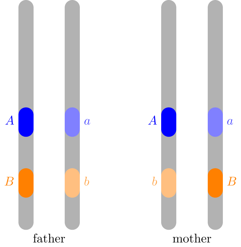
Exercise 13.3 (Linkage and recombination) Consider two parents who are carriers of the recessive alleles for two genes \(A\) and \(B\) on the same chromosome, as in Example 13.2. However, the father has \(A\) and \(B\) on one chromosome, while the mother has \(A\) and \(b\) on one chromosome, as shown below. Assume that the recombination probability is \(p\).
Let \(X\) be the number of dominant \(A\) alleles and \(Y\) be the number of dominant \(B\) alleles in the child.
- Calculate the joint PMF of \(X\) and \(Y\) in terms of \(p\).
- Calculate the marginal PMFs of \(X\) and \(Y\), and comment on whether they make sense.
Exercise 13.4 (Predicting Tennis) You have built a model predicting the outcomes of tennis matches. Suppose we are trying to predict how Aryna Sabalenka and Iga Swiatek will perform in the U.S. Open, starting from the round of 8.
Let \(X\) be the number of games Sabalenka wins during the match and \(Y\) be the number of games Swiatek wins during the match. Your model predicts the following:
| \(0\) |
\(0.12\) |
\(0.112\) |
\(0.0504\) |
\(0.1176\) |
| \(1\) |
\(0.054\) |
\(0.0504\) |
\(0.02268\) |
\(0.05292\) |
| \(2\) |
\(0.0504\) |
\(0.04704\) |
\(0\) |
\(0.10584\) |
| \(3\) |
\(0.0756\) |
\(0.07056\) |
\(0.07056\) |
\(0\) |
- What do \(P(X = 2, Y = 2) = P(X = 3, Y = 3) = 0\) seem to indicate?
- Calculate the marginal PMF of \(X\) and \(Y\). Are \(X\) and \(Y\) independent?
- Compute \(P(X = 3 \mid Y = 2)\) and \(P(Y = 3 \mid X = 2)\). Should they sum to \(1\)? Why or why not?