33 Convolutions

In the introduction, we discussed the general goal of this part, which is to characterize the sampling distribution of estimators of the form \[ g\left( \sum_{i=1}^n X_i \right). \] As the first step towards this goal, we first discuss how to calculate the sampling distribution of \[ S_n = \sum_{i=1}^n X_i, \] a sum of $n$ independent random variables. The sample mean $\bar X$ only differs from $S_n$ by a scale transformation, so its sampling distribution is also straightforward to derive, once we have the distribution of $S_n$.

33.1 Discrete Convolutions

The process used to determine the distribution of a sum of independent random variables is called convolution. Convolution operates on two random variables at a time. That is, to determine the distribution of $S_n = \sum_{i=1}^n X_i$,

we first determine the distribution of $S_2 = X_1 + X_2$,
then determine the distribution of $S_3 = (X_1 + X_2) + X_3 = S_2 + X_3$,
then determine the distribution of $S_4 = (X_1 + X_2 + X_3) + X_4 = S_3 + X_4$,

and so on. Once we know how to calculate the distribution of the sum of two independent random variables, we can calculate the distribution of the sum of any number of independent random variables by simply iterating the process.

Let $X$ and $Y$ be independent discrete random variables with PMFs $f_X(x)$ and $f_Y(y)$, respectively. The method for determining the PMF of $S = X + Y$ is straightforward in theory but difficult in practice.

Since the PMF of $S$ is \[ f_S(s) = P(S = s) = P(X + Y = s), \] we just need to evaluate this probability for all possible values of $s$. When $X$ and $Y$ are both integer-valued, the event $\left\{ X + Y = s \right\}$ can be expressed as a disjoint union of all the different possible values of $X$ and $Y$ that add up to $s$: \[ \cdots \cup \left\{ X = 0, Y = s \right\} \cup \left\{ X = 1, Y = s-1 \right\} \cup \left\{ X = 2, Y = s-2 \right\} \cup \cdots. \]

Therefore, the PMF of $S$ is \[ \begin{align*} f_S(s) = P(X + Y = s) &= \sum_{x = -\infty}^\infty P(X = x, Y = s-x) \\ &= \sum_{x=-\infty}^\infty P(X = x) P(Y = s - x) \\ &= \sum_{x=-\infty}^\infty f_X(x) f_Y(s - x), \end{align*} \] where we used independence of $X$ and $Y$ in the second step.

This recipe is summarized in the following theorem.

Theorem 33.1 (Discrete convolution) Let $X$ and $Y$ be independent discrete random variables with PMFs $f_X(x)$ and $f_Y(y)$, respectively. Then, the PMF of $S = X + Y$ is \[ f_S(s) = \sum_x f_X(x) f_Y(s - x). \tag{33.1}\]

The function $f_S$ is said to be the discrete convolution of the functions $f_X$ and $f_Y$ and is denoted \[ f_S = f_X * f_Y. \]

We now apply Theorem 33.1 to an example.

Example 33.1 (Sum of independent Poissons) Let $X \sim \text{Poisson}(\mu_1)$ and $Y \sim \text{Poisson}(\mu_2)$ be independent. What is the distribution of $S = X+Y$?

The possible values of $X$ and $Y$ are $0, 1, 2, \dots$, so the possible values of $S$ are also $0, 1, 2, \dots$. Fix an integer $s \geq 0$. Then, in order for the sum of $X$ and $Y$ to equal $s$, $X$ cannot be greater than $s$. \[ \begin{align*} f_S(s) &= \sum_{x=0}^s f_X(x) f_Y(s - x) \\ &= \sum_{x=0}^s \left( \frac{\mu_1^x e^{-\mu_1}}{x!} \right) \left( \frac{\mu_2^{s-x} e^{-\mu_2}}{(s-x)!} \right) \\ &= \sum_{x=0}^s e^{-\mu_1 - \mu_2} \frac{\mu_1^x \mu_2^{s-x}}{x!(s-x)!} \\ &= e^{-\mu_1 - \mu_2} \sum_{x=0}^s \frac{1}{x!(s-x)!} \mu_1^x \mu_2^{s-x} \\ &= e^{-\mu_1 - \mu_2} \sum_{x=0}^s \frac{s!}{x!(s-x)!} \frac{\mu_1^x \mu_2^{s-x}}{s!} \\ &= e^{-\mu_1 - \mu_2} \sum_{x=0}^s \binom{s}{x} \frac{\mu_1^x \mu_2^{s-x}}{s!} \\ &= \frac{e^{-\mu_1 - \mu_2}}{s!} \sum_{x=0}^s \binom{s}{x} \mu_1^x \mu_2^{s-x} \\ &= \frac{e^{-\mu_1 - \mu_2}}{s!} (\mu_1 + \mu_2)^s, \end{align*}\] which is the PMF of $\text{Poisson}(\mu_1 + \mu_2)$. Thus, \[ S = X+Y \sim \text{Poisson}(\mu_1 + \mu_2). \]

In other words, the sum of two independent Poissons is another Poisson random variable whose parameter is the sum of the individual parameters. An immediate consequence of Example 33.1 is that if $X_1, \dots, X_n$ are i.i.d. $\text{Poisson}(\mu)$, then \[ X_1 + \cdots + X_n \sim \text{Poisson}(n \mu). \]

33.2 Continuous Convolutions

Let $X$ and $Y$ be independent continuous random variables. The process of finding the PDF of $S = X+Y$ is similar to Theorem 33.1, except with PMFs replaced by PDFs and sums replaced by integrals.

Theorem 33.2 (Continuous convolution) Let $X$ and $Y$ be independent continuous random variables with PDFs $f_X(x)$ and $f_Y(y)$, respectively. Then, the PDF of $S = X + Y$ is \[ f_S(s) = \int_{-\infty}^\infty f_X(x) f_Y(s - x)\,dx. \tag{33.2}\]

The function $f_S$ is said to be the convolution of the functions $f_X$ and $f_Y$ and is denoted \[ f_S = f_X * f_Y. \]

Proof

In Chapter 20, we discussed a general way to find the distribution of a transformed random variable. We apply that same recipe here:

Compute the CDF $F_S(s)$
Differentiate (with respect to $s$) to get the PDF $f_S(s)$.

Once we have the PDF, we can compute probabilities related to $S = X + Y$. In general, \[\begin{align*} F_S(s) &= P(X + Y \leq s) \\ &= \iint_{\{x+y \leq s\}} f_{X,Y}(x,y) \, dy \, dx \\ &= \iint_{\{x+y \leq s\}} f_X(x) f_Y(y) \, dy \, dx \qquad \qquad \text{($X$ and $Y$ are independent)} \\ &= \int_{-\infty}^\infty \int_{-\infty}^{s-x} f_X(x) f_Y(y) \, dy \, dx \\ &= \int_{-\infty}^\infty f_X(x) \int_{-\infty}^{s-x} f_Y(y) \, dy \, dx \\ &= \int_{-\infty}^\infty f_X(x) \left( F_Y(y) \right) \Biggr|_{-\infty}^{s-x} \, dx \\ &= \int_{-\infty}^\infty f_X(x) F_Y(s-x) \, dx. \end{align*}\]

Now, we differentiate $F_S$ to obtain the PDF $f_S$. \[\begin{align*} f_S(s) &= \frac{d}{ds} \int_{-\infty}^\infty f_X(x) F_Y(s-x) \, dx \\ &= \int_{-\infty}^\infty f_X(x) \frac{d}{ds} F_Y(s-x) \, dx \\ &= \int_{-\infty}^\infty f_X(x) f_Y(s-x) \, dx. \end{align*}\]

Now we apply Theorem 33.2 to several examples. The first example is a step towards deriving the sampling distribution of the MLE from Example 30.3.

Example 33.2 (Sum of independent standard normals) Let $Z$ and $W$ be i.i.d. $\textrm{Normal}(\mu= 0, \sigma^2= 1)$. What is the distribution of $S = Z + W$?

By Theorem 33.2, we calculate \[ \begin{align*} f_S(s) &= \int_{-\infty}^\infty f_Z(z) f_W(s-z) \, dz \\ &= \int_{-\infty}^\infty \left( \frac{1}{\sqrt{2\pi}} \exp\left\{ -\frac{z^2}{2} \right\} \right) \left( \frac{1}{\sqrt{2\pi}} \exp \left\{ -\frac{(s-z)^2}{2} \right\} \right) \, dz \\ &= \int_{-\infty}^\infty \frac{1}{2\pi} \exp \left\{ -\frac{z^2}{2} - \frac{(s-z)^2}{2} \right\} \, dz \\ &= \frac{1}{2\pi} \int_{-\infty}^\infty \exp \left\{ - \frac{2z^2 - 2sz + s^2}{2} \right\} \, dz \\ &= \frac{1}{2\pi} \exp\left\{ -\frac{s^2}{2} \right\} \int_{-\infty}^\infty \exp \left\{ - \frac{2 (z^2 - sz + \frac{s^2}{4}) }{2} \right\} \exp \left\{ \frac{s^2}{4} \right\} \, dz \\ &= \frac{1}{\sqrt{2\pi \cdot 2}} \exp \left\{ -\frac{s^2}{4} \right\} \int_{-\infty}^\infty \underbrace{\frac{1}{\sqrt{2\pi \cdot \frac{1}{2}}} \exp \left\{ -\frac{1}{2 \cdot \frac{1}{2}} \left( z - \frac{s}{2} \right)^2 \right\} }_{\text{PDF of $\textrm{Normal}(\mu= \frac{s}{2}, \sigma^2= \frac{1}{2})$}} \, dz \\ &= \frac{1}{\sqrt{2\pi \cdot 2}} \exp \left\{ -\frac{s^2}{2 \cdot 2} \right\} \end{align*} \] which is the PDF of $\textrm{Normal}(\mu= 0, \sigma^2= 2)$. Hence, \[ S = Z + W \sim \textrm{Normal}(\mu= 0, \sigma^2= 2). \]

We can check this result by simulation.

Now, if $X_1$ and $X_2$ are i.i.d. normal random variables with mean $\mu$ and variance $\sigma^2$, then their sample mean is \[ \bar X = \frac{X_1 + X_2}{2} = \frac{(\mu + \sigma Z) + (\mu + \sigma W)}{2} = \mu + \frac{\sigma}{2} S, \] which is just a location-scale transformation (Definition 20.1) of $S$. We know that a location-scale transformation of a normal random variable is also normal, so \[ \bar X \sim \text{Normal}(\mu, \frac{\sigma^2}{2}). \]

In principle, the above calculation can be extended to obtain the sampling distribution of a sample mean of $n$ i.i.d. normal random variables. However, the algebra is quite messy, so we will defer this result to Example 34.7, when we have developed a simpler way to identify the distribution of a sum of independent random variables.

When applying Theorem 33.2, we often need to be mindful of the support of the distributions, as the next example illustrates.

Example 33.3 (Sum of independent uniforms) Let $X$ and $Y$ be independent $\textrm{Uniform}(a= 0, b= 1)$. What is the distribution of $S = X + Y$?

First, let’s get a feel for this distribution by simulation. Can you explain intuitively why $S$ has this distribution.

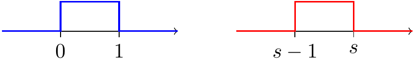
Now, let’s calculate the distribution. By Theorem 33.2, \[ f_S(s) = \int_{-\infty}^\infty f_X(x) f_Y(s-x) \, dx. \] Since both $f_X(x)$ and $f_Y(s-x)$ take values 0 or 1, their product is also either 0 or 1. The integrand equals 1 only when both $f_X(x)$ and $f_Y(s-x)$ are simultaneously 1—that is, when their supports overlap. The nature of this overlap depends on the value of $s$. To visualize this, we start with the following representations of $\color{blue}f_X(x)$ and $\color{red}f_Y(s-x)$:

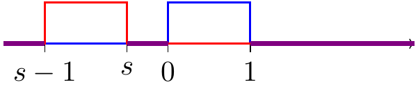
The supports of $\color{blue}f_X(x)$ and $\color{red}f_Y(s-x)$ do not intersect when $s < 0$:

or when $s > 2$:

Hence, for $s < 0$ or $s > 2$, \[ f_X(x) f_Y(s-x) = 0, \] so $f_S(s) = 0$.

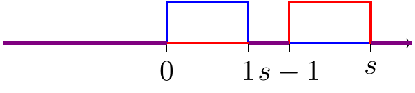
When the supports do overlap, there are two distinct cases. The first is when $0 < s < 1$:

The supports overlap between $0$ and $s$, and thus, \[ f_S(s) = \int_{-\infty}^\infty f_X(x) f_Y(s-x) \, dx = \int_0^s \, dx = s \] for $0 < s < 1$. The other case is when $1 < s < 2$:

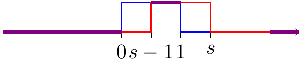
The supports overlap between $s-1$ and $1$, so \[ f_S(s) = \int_{-\infty}^\infty f_X(x) f_Y(s-x) \, dx = \int_{s-1}^1 \, dx = 2-s \] for $1 < s < 2$.

Combining all cases, the PDF of $S$ is \[ f_S(s) = \begin{cases} s, & 0 < s < 1 \\ 2-s, & 1< s < 2 \\ 0, & \text{otherwise} \end{cases}. \]

This corresponds to the triangular distribution shown below.

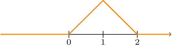
Figure 33.6: Distribution of a sum of two independent $\textrm{Uniform}(a= 0, b= 1)$ random variables.

This agrees with our simulation.

In the last example, we demonstrate how to use convolutions on random variables with possibly different distributions. This will allow us to derive the sampling distribution of the MLE from Example 32.4.

Example 33.4 (Sum of independent exponentials) Let $X$ and $Y$ be independent $\text{Exponential}(\lambda)$. We first calculate the density of $S = X+Y$.

By Theorem 33.2, for $s > 0$, \[\begin{align*} f_S(s) &= \int_{-\infty}^\infty f_X(x) f_Y(s-x) \, dx \\ &= \int_0^s f_X(x) f_Y(s-x) \, dx & (\text{$f_S(x) = 0$ for $x < 0$ and $f_Y(s-x) = 0$ for $x > s$}) \\ &= \int_0^s \left( \lambda e^{-\lambda x} \right) \left( \lambda e^{-\lambda (s-x)} \right) \, dx \\ &= \int_0^s \lambda^2 e^{-\lambda s} \, dx \\ &= \lambda^2 s e^{-\lambda s}. \end{align*}\]

What happens if we add a third exponential? Let $W \sim \text{Exponential}(\lambda)$ be independent of $X$ and $Y$ (and thus of $S$). What is the density of $T = X+Y+W = S+W$? Now, we are adding two random variables with different distributions. The process is the same. By Theorem 33.2, for $t > 0$, \[ \begin{align*} f_T(t) &= \int_{-\infty}^\infty f_S(s) f_W(t-s) \, ds \\ &= \int_0^t f_S(s) f_W(t-s) \, ds & (\text{$f_S(s) = 0$ for $s < 0$ and $f_W(t - s) = 0$ for $s > t$}) \\ &= \int_0^t \left( \lambda^2 s e^{-\lambda s} \right) \left( \lambda e^{-\lambda (t - s)} \right) \, ds \\ &= \int_0^t \lambda^3 s e^{-\lambda t} \, ds \\ &= \lambda^3 e^{-\lambda t} \int_0^t s \, ds \\ &= \frac{\lambda^3}{2} t^2 e^{-\lambda t}. \end{align*}\]

Therefore, the MLE from Example 32.4, $\bar X$, has the following sampling distributions for $n=\textcolor{blue}{2}$ and $n=\textcolor{red}{3}$: \[ \begin{align} f_{\textcolor{blue}{\bar X_2}}(x) = f_{S/2}(x) &= 2 f_S(2x) = 4\lambda^2 x e^{-2\lambda x} \\ f_{\textcolor{red}{\bar X_3}}(x) = f_{T/3}(x) &= 3 f_T(3x) = \frac{27\lambda^3}{2} x^2 e^{-3\lambda x}. \end{align} \] These densities are graphed below, along with the PDF of $X_1$, assuming $\lambda = 1$.

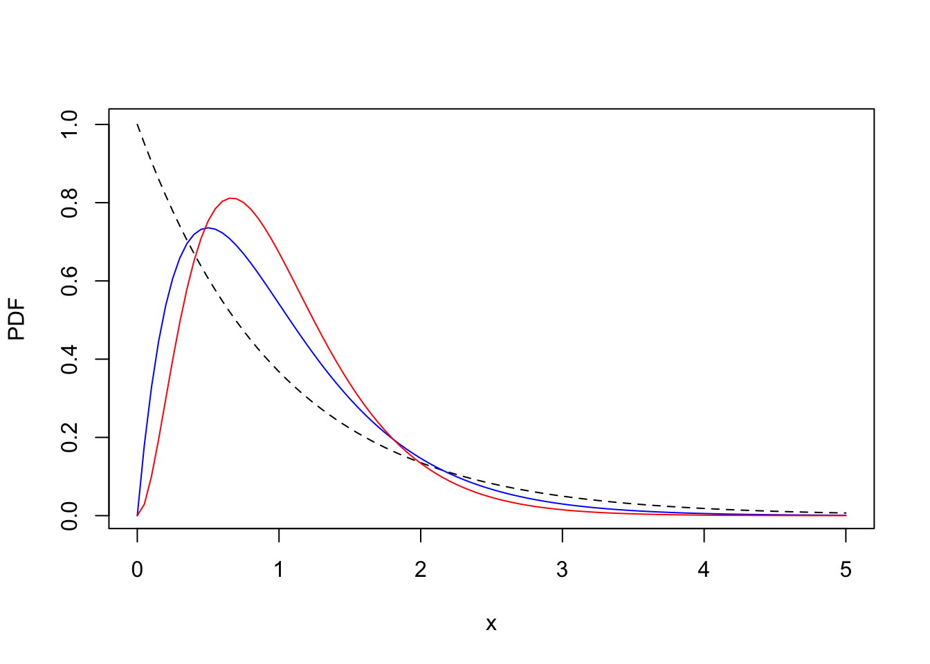
Even for these small values of $n$, the sampling distribution appears to concentrate around $\mu = \frac{1}{\lambda}$ (which equals $1$ in the plot above). With explicit PDFs for the sampling distribution, we can calculate the probability that the estimate is within $10\%$ of the true value.

\[ \begin{align} P(0.9\mu < \textcolor{blue}{\bar X_2} < 1.1\mu) &= \int_{0.9 \mu}^{1.1 \mu} \frac{4}{\mu^2} x e^{-2x / \mu} \, dx \approx 0.108 \\ P(0.9\mu < \textcolor{red}{\bar X_3} < 1.1\mu) &= \int_{0.9 \mu}^{1.1 \mu} \frac{27}{2\mu^3} x^2 e^{-3x / \mu} \, dx \approx 0.134. \end{align} \]

We might be interested in how this probability increases with $n$. We could determine the sampling distribution of $\bar X_n$ by repeated convolution; Exercise 33.6 asks you to supply the details. However, in Chapter 36, we will calculate an accurate approximation to the distribution of $\bar X_n$ for large values of $n$, and in Chapter 38, we will obtain an exact formula for its distribution as part of a more general theory.

33.3 Exercises

Exercise 33.1 (Distribution of a difference) Let $X$ and $Y$ be independent continuous random variables. Show that \[ f_{X-Y}(z) = \int_{-\infty}^\infty f_X(x) f_Y(x-z) \, dx. \]

Exercise 33.2 (Binomial convolution) Let $X \sim \text{Binomial}(n,p)$ and $Y \sim \text{Binomial}(m,p)$ be independent.

Use convolution to determine the distribution of $S = X+Y$. Explain why the result makes sense intuitively.
Explain why Example 33.1 is not surprising in light of this result.

Exercise 33.3 (Negative binomial convolution) Let $X \sim \text{NegativeBinomial}(r,p)$ and $Y \sim \text{NegativeBinomial}(s,p)$ be independent. Use convolution to determine the distribution of $S = X+Y$.

Explain why the result makes sense intuitively.

Exercise 33.4 (Sum of i.i.d. uniforms) Let $X, Y, Z$ be i.i.d. $\textrm{Uniform}(a= 0, b= 1)$. What is the distribution of $S_3 = X + Y + Z$?

Hint: Make use of what we derived above.

Exercise 33.5 (Sum of different uniforms) Let $X \sim \textrm{Uniform}(a= 0, b= 1)$ and $Y \sim \textrm{Uniform}(a= -1, b= 2)$ be independent. What is the distribution of $S = X+Y$?

Exercise 33.6 (Sum of exponentials by induction) Using induction, derive a general formula for the PDF of $S_n = X_1 + \dots + X_n$, where $X_i$ are i.i.d. $\text{Exponential}(\lambda)$. Note that $n = 2, 3$ were already done in Example 33.4.

Exercise 33.7 (Difference of exponentials) In Example 24.1, we modeled the times that two people enter an amusement park as independent random variables $X \sim \text{Exponential}(\lambda_1)$ and $Y \sim \text{Exponential}(\lambda_2)$ and calculated $\text{E}\!\left[ |X - Y| \right]$, the expected time that the first person to arrive has to wait for the other person to arrive.

Now, determine the PDF of $X - Y$, and use this PDF to calculate $\text{E}\!\left[ |X - Y| \right]$. Verify that your answer matches Example 24.1.