11 LotUS and Variance

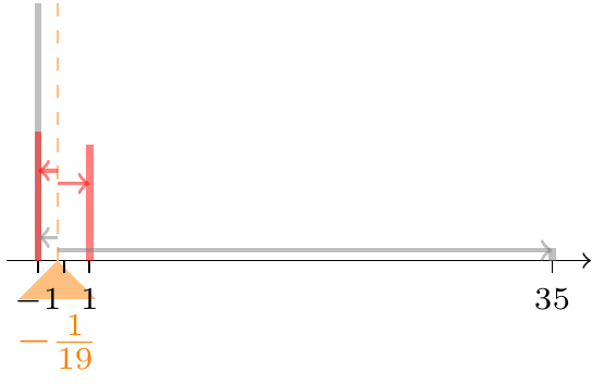
In Example 9.2, we saw that a $1 bet on a single number and a $1 bet on red in roulette have the same expected profit of $-\frac{1}{19}$. However, the two bets are very different; we need summaries of a random variable that help us decide between these two bets. In particular, we will develop summaries of the form $\text{E}\!\left[ g(X) \right]$, where $g$ is a suitably chosen function.

11.1 Law of the Unconscious Statistician

How do we calculate $\text{E}\!\left[ g(X) \right]$? To be concrete, suppose as in Example 10.2 that $X$ is the price of a stock next week, and we want to calculate the expected value of a call option to buy the stock at a strike price of $55: \[ \text{E}\!\left[ \max(X - 55, 0) \right]. \]

One way to calculate this expectation is suggested by Chapter 10:

Determine the PMF of $Y \overset{\text{def}}{=}\max(X - 55, 0)$.
Calculate $\text{E}\!\left[ Y \right]$ using Definition 9.1.

However, there is another way, if we appeal to the idea of the expected value as a weighted average.

Example 11.1 (Expected value of a call option) To calculate $\text{E}\!\left[ X \right]$, we weight the values of $X$ by their probabilities. To calculate $\text{E}\!\left[ \max(X - 55, 0) \right]$, we can simply weight the values of $\max(X - 55, 0)$ by the same probabilities. That is, using the PMF of $X$ from Example 10.2, we have \[ \begin{align} \text{E}\!\left[ \max(X - 55, 0) \right] &= \max(50 - 55, 0) \cdot \frac{1}{8} + \max(53 - 55, 0) \cdot \frac{2}{8} \\ &\quad \quad + \max(57 - 55, 0) \cdot \frac{4}{8} + \max(60 - 55, 0) \cdot \frac{1}{8} \\ &= 0 \cdot \frac{1}{8} + 0 \cdot \frac{2}{8} + 2 \cdot \frac{4}{8} + 5 \cdot \frac{1}{8} \\ &= \$1.625. \end{align} \]

To check this answer, we can use the PMF of $Y = \max(X - 55, 0)$ that we derived in Example 10.2: \[ \text{E}\!\left[ Y \right] = 0 \cdot \frac{3}{8} + 2 \cdot \frac{4}{8} + 5 \cdot \frac{1}{8} = \$1.625. \]

The fact that the two ways of calculating $\text{E}\!\left[ g(X) \right]$ agree is a theorem, even though it is intuitive from the definition of expected value. Because many statisticians forget that this fact requires proof, it is sometimes called the “Law of the Unconscious Statistician.”

Theorem 11.1 (Law of the Unconscious Statistician (LotUS)) Let $X$ be a discrete random variable with PMF $f_X$. Then, \[ \text{E}\!\left[ g(X) \right] = \sum_x g(x) f_X(x), \tag{11.1}\] where the sum is over the possible values of $X$.

Proof

Since $Y = g(X)$ is itself a random variable, its expected value is defined as \[ \text{E}\!\left[ g(X) \right] = \text{E}\!\left[ Y \right] = \sum_y y f_Y(y). \]

Recall how we found the PMF of $Y$ using Equation 10.3. For each possible value of $Y$, we sum the probabilities of the corresponding values of $X$: \[ f_Y(y) = \sum_{x: g(x) = y} f_X(x). \]

Substituting this into the expression above, we obtain \[ \begin{align} \text{E}\!\left[ g(X) \right] &= \sum_y y \sum_{x: g(x) = y} f_X(x) \\ &= \sum_y \sum_{x: g(x)=y} g(x) f_X(x) \\ &= \sum_x g(x) f_X(x). \end{align} \]

The last line follows because the sets $B_y = \{ x: g(x) = y \}$ represent a partition of the possible values of $x$.

LotUS is the workhorse that powers Daniel Bernoulli’s expected utility theory, which he developed to resolve the St. Petersburg Paradox (Example 9.6).

Example 11.2 (St. Petersburg Paradox and expected utility) In Example 9.6, we described a game whose payout $X$ had an infinite expected value, which implies that we should be willing to pay any amount of money to play this game.

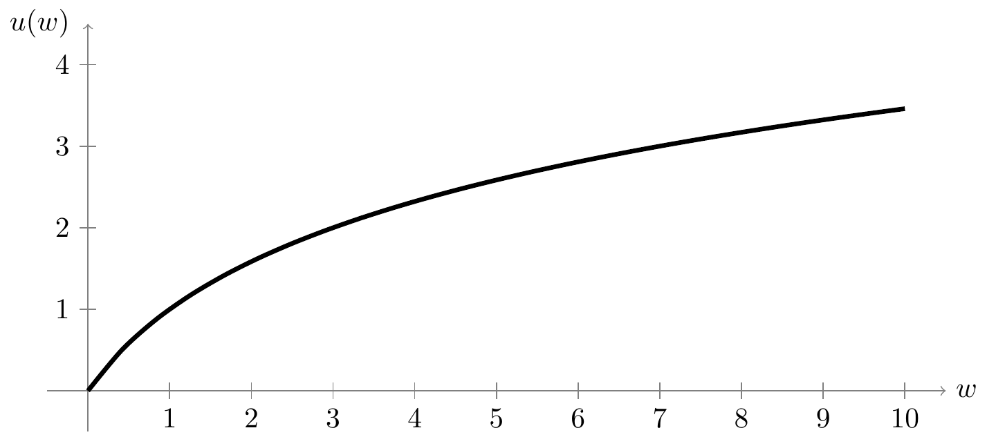
Daniel Bernoulli resolved this paradox by arguing that what matters is not the payout $X$, but the utility (or “satisfaction”) that we derive from that payout. Because we derive less utility from each additional dollar (an extra dollar means a lot if you only have $10, but not if you are a billionaire), the utility function $u(w)$ is concave, a property that economists call diminishing marginal utility. An example of a typical utility function is shown in Figure 11.1.

Figure 11.1: A concave utility function.

Suppose your utility function is \[ u(w) = \log(w) \] and your current wealth is $100. Then, your options are:

don’t play this game, in which case your utility is $u(100) \approx 4.605$ “utils” (the units for utility), or
pay $\$c$ to play this game, in which case your utility is $u(100 - c + X)$.

Bernoulli’s theory says that you should be willing to pay $$c$ to play if your
expected utility is greater than your utility if you do not play the game: \[ \text{E}\!\left[ u(100 - c + X) \right] > u(100). \]

To calculate the expected utility, we apply LotUS (Theorem 11.1) to the PMF of $X$ derived in Example 9.6: \[ \begin{align} \text{E}\!\left[ \log(100 - c + X) \right] &= \sum_{x} \log(100 - c + x) f_X(x) \\ &= \log(101 - c) \cdot \frac{1}{2} + \log(102 - c) \cdot \frac{1}{4} + \log(104 - c) \cdot \frac{1}{8} + \ldots \end{align} \] Although this sum does not have a simple closed-form expression, it is at least finite (for any $0 < c < 100$), unlike $\text{E}\!\left[ X \right]$.

Proof that infinite series converges

The expected utility can be written as the infinite series \[ \sum_{n=1}^\infty \frac{\log(100 - c + 2^{n-1})}{2^n}, \] and we can bound $100 - c + 2^{n-1}$ by $2^7 + 2^n < 2^{n+7}$ for $n \geq 1$, so \[ \sum_{n=1}^\infty \frac{\log(100 - c + 2^{n-1})}{2^n} < \sum_{n=1}^\infty \frac{\log(2^{n+7})}{2^n} = \log(2) \sum_{n=1}^\infty \frac{n+7}{2^n}. \] Now, we can use d’Alembert’s ratio test to see that the series on the right-hand side converges: \[ \left| \frac{a_{n+1}}{a_n} \right| < \left| \frac{\frac{n+8}{2^{n+1}}}{\frac{n+7}{2^{n}}} \right| = \frac{n+8}{n+7} \frac{1}{2} \to \frac{1}{2} < 1. \]

Because the series converges, we can approximate its value by summing the first few terms. The code below calculates the expected utility for a particular value of $c$. Try changing $c$. For what values of $c$ is this expected utility greater than the $4.605$ utils if you do not play the game?

Expected utility theory suggests that we should only be willing to pay about $4.62 to play this game!

We can also use expected utility to distinguish between the two roulette bets.

Example 11.3 (Roulette and expected utility) Consider a gambler whose utility function is $u(w) = \sqrt{w}$. If they brought $10 to the casino, should they bet $1 on a single number or $1 on reds? In Example 9.2, we saw that the two bets had exactly the same expected profit of $\text{E}\!\left[ \S \right] = \text{E}\!\left[ \RR \right] = \$-1/19$.

However, the two bets have different expected utilities.

The bet on a single number has an expected utility of \[ \begin{align} \text{E}\!\left[ u(10 + \S) \right] &= u(10 - 1) \cdot \frac{37}{38} + u(10 + 35) \cdot \frac{1}{38} \\ &= \sqrt{10 - 1} \cdot \frac{37}{38} + \sqrt{10 + 35} \cdot \frac{1}{38} \\ &= 3.098, \end{align} \] while the bet on reds has an expected utility of \[ \begin{align} \text{E}\!\left[ u(10 + \RR) \right] &= u(10 - 1) \cdot \frac{20}{38} + u(10 + 1) \cdot \frac{18}{38} \\ &= \sqrt{10 - 1} \cdot \frac{20}{38} + \sqrt{10 + 1} \cdot \frac{18}{38} \\ &= 3.145. \end{align} \]

Therefore, the bet on reds has a higher expected utility.

Caution!

Example 11.3 reminds us that \[ \text{E}\!\left[ g(X) \right] \neq g(\text{E}\!\left[ X \right]). \]

We saw that $\text{E}\!\left[ u(10 - \RR) \right] = 3.145$, which is different from the answer we get if we plug in the expected value into the utility function: $u(10 - \text{E}\!\left[ \RR \right]) = \sqrt{10 - (-\frac{1}{19})} = 3.171$.

There is one situation where we can simply plug in the expected value into the transformation $g$—when it is linear, of the form \[ g(X) = aX + b. \] In these situations, we can bypass LotUS.

Proposition 11.1 (Expected value of a linear transformation) Let $X$ be a random variable and let $a$ and $b$ be constants. Then,

\[\text{E}\!\left[ aX + b \right] = a \text{E}\!\left[ X \right] + b \tag{11.2}\]

Proof

By LotUS, \[ \begin{aligned} \text{E}\!\left[ aX + b \right] &= \sum_x (ax + b) f_X(x) & \text{(LotUS)} \\ &= \sum_x ax f_X(x) + \sum_x b f_X(x) & \text{(split up sum)} \\ &= a \underbrace{\sum_x x f_X(x)}_{\text{E}\!\left[ X \right]} + b \underbrace{\sum_x f_X(x)}_1 & \text{(pull out constants)} \\ &= a \text{E}\!\left[ X \right] + b. \end{aligned} \] In the last step, we used the fact that any PMF sums to 1.

When the transformation is linear, applying Proposition 11.1 is much easier than applying LotUS.

Example 11.4 (Roulette and linear transformations) In Example 10.1, we saw that $\S = 36 I - 1$, where $I$ is a $\text{Bernoulli}(p=\frac{1}{38})$ random variable. Since we already know by Proposition 9.2 that $\text{E}\!\left[ I \right] = \frac{1}{38}$, we can use Proposition 11.1 to conclude that \[ \text{E}\!\left[ \S \right] = 36 \text{E}\!\left[ I \right] - 1 = 36 \cdot \frac{1}{38} - 1 = -\frac{1}{19}. \]

However, Example 11.4 is more the exception than the rule. In general, LotUS is the foolproof way to calculate an expectation of the form $\text{E}\!\left[ g(X) \right]$.

11.2 Variance

Another difference between the two roulette bets is how much their outcomes vary. This is captured by the variance, which measures how much the possible outcomes differ from the expected value, as illustrated in Figure 11.2.

Figure 11.2: The variance measures how much the values deviate from the expected value of $-1/19$. It is clear that $\S$ has a larger variance than $\RR$.

Definition 11.1 (Variance of a discrete random variable) Let $X$ be a discrete random variable. Then, the variance of $X$ is \[ \text{Var}\!\left[ X \right] \overset{\text{def}}{=}\text{E}\!\left[ (X - \text{E}\!\left[ X \right])^2 \right]. \tag{11.3}\]

We can use Equation 11.3 to calculate the variance of the different roulette bets.

Example 11.5 (Variance of roulette bets) Let $\S$ be the profit from a $1 bet on a single number. Then $\text{E}\!\left[ \S \right] = -\frac{1}{19}$.

The variance is \[ \begin{aligned} \text{Var}\!\left[ \S \right] &= \text{E}\!\left[ (\S - \text{E}\!\left[ \S \right])^2 \right] \\ &= \sum_x (x - (-\frac{1}{19}))^2 \cdot f_{\S}(x) \\ &= (35 - (-\frac{1}{19}))^2 \cdot \frac{1}{38} + (-1 - (-\frac{1}{19}))^2 \cdot \frac{37}{38} \\ &\approx 33.2078. \end{aligned} \]

Now let $\RR$ be the profit from a $1 bet on reds. Then $\text{E}\!\left[ \RR \right] = -\frac{1}{19}$ and the variance is \[ \begin{aligned} \text{Var}\!\left[ \RR \right] &= \text{E}\!\left[ (\RR - \text{E}\!\left[ \RR \right])^2 \right] \\ &= \sum_x (x - (-\frac{1}{19}))^2 \cdot f_{\RR}(x) \\ &= (1 - (-\frac{1}{19}))^2 \cdot \frac{18}{38} + (-1 - (-\frac{1}{19}))^2 \cdot \frac{20}{38} \\ &\approx 0.9972. \end{aligned} \]

So the bet on a single number has a much larger variance than the bet on reds. This can be a good or a bad thing, depending on whether the gambler prefers to live on the edge or play it safe.

What are the units of variance? In Example 11.5, $\RR$ was measured in dollars, so $\text{Var}\!\left[ \RR \right]$ is measured in squared dollars. Because it is often difficult to interpret squared units, it is common to instead report the square root of variance, which is in the same units as the original random variable.

Definition 11.2 (Standard deviation of a discrete random variable) Let $X$ be a discrete random variable. Then, the standard deviation of $X$ is \[ \text{SD}\!\left[ X \right] \overset{\text{def}}{=}\sqrt{\text{Var}\!\left[ X \right]}. \tag{11.4}\]

The standard deviations of Example 11.5 are \[ \begin{align} \text{SD}\!\left[ \S \right] &\approx \sqrt{33.2078} \approx \$5.76 & \text{SD}\!\left[ \RR \right] &\approx \sqrt{0.9972} \approx \$0.999, \end{align} \] and note that these standard deviations represent dollar amounts.

There is another version of the variance formula that is often easier for computations.

Proposition 11.2 (Shortcut Formula for Variance) \[ \text{Var}\!\left[ X \right] = \text{E}\!\left[ X^2 \right] - (\text{E}\!\left[ X \right])^2 \tag{11.5}\]

Proof

Let $\mu = \text{E}\!\left[ X \right]$. Note that $\mu$ is a constant.

Using LotUS, we can expand the term inside the sum to obtain the shortcut formula. \[ \begin{align*} \text{Var}\!\left[ X \right] &= \text{E}\!\left[ (X - \mu)^2 \right] \\ &= \sum_x (x-\mu)^2 f_X(x) \\ &= \sum_x (x^2 - 2\mu x + \mu^2) f_X(x) \\ &= \underbrace{\sum_x x^2 f_X(x)}_{\text{E}\!\left[ X^2 \right]} - 2 \mu \underbrace{\sum_x x f_X(x)}_{\text{E}\!\left[ X \right]} + \mu^2 \underbrace{\sum_x f_X(x)}_1 \\ &= \text{E}\!\left[ X^2 \right] - 2\mu \text{E}\!\left[ X \right] + \mu^2 \\ &= \text{E}\!\left[ X^2 \right] - 2\mu^2 + \mu^2 \\ &= \text{E}\!\left[ X^2 \right] - (\text{E}\!\left[ X \right])^2. \end{align*} \]

The shortcut formula is easier because usually $\text{E}\!\left[ X \right]$ is already known, so only $\text{E}\!\left[ X^2 \right]$ needs to be computed. Let’s apply the shortcut formula to the roulette example from Example 11.5.

Example 11.6 (Variance of roulette bets with the shortcut formula) For the bet on a single number, we know that $\text{E}\!\left[ \S \right] = -\frac{1}{19}$ so we just need to compute $\text{E}\!\left[ \S^2 \right]$ using LotUS: \[ \text{E}\!\left[ \S^2 \right] = (35)^2 \cdot \frac{1}{38} + (-1)^2 \cdot \frac{37}{38} = \frac{631}{19}. \] By Proposition 11.2, the variance is \[ \text{Var}\!\left[ \S \right] = \text{E}\!\left[ \S^2 \right] - (\text{E}\!\left[ \S \right])^2 = \frac{631}{19} - (-\frac{1}{19})^2 \approx 33.2078.\]

For the bet on reds, we know that $\text{E}\!\left[ \RR \right] = -\frac{1}{19}$. To calculate $\text{E}\!\left[ \RR^2 \right]$, we could use LotUS again, or we could simply observe that $\RR^2 = 1$ (since $\RR$ is either $-1$ or $1$), so $\text{E}\!\left[ \RR^2 \right] = 1$.

By Proposition 11.2, the variance is \[ \text{Var}\!\left[ \RR \right] = \text{E}\!\left[ \RR^2 \right] - (\text{E}\!\left[ \RR \right])^2 = 1 - (-\frac{1}{19})^2 \approx 0.9972.\] These answers match the ones we obtained in Example 11.5.

In Proposition 9.2, we determined the expectation of a $\text{Binomial}(n,p)$ random variable $X$ to be $\text{E}\!\left[ X \right] = np$. Now, we will use Proposition 11.2 to derive a similar expression for $\text{Var}\!\left[ X \right]$.

Proposition 11.3 (Variance of a binomial) Let $X \sim \text{Binomial}(n,p)$. Then, \[ \text{E}\!\left[ X \right] = np(1 - p). \]

Proof

First, we use LotUS to calculate $\text{E}\!\left[ X^2 \right]$:

\[ \begin{align*} \text{E}\!\left[ X^2 \right] &= \sum_{x=0}^n x^2 \binom{n}{x} p^x (1-p)^{n-x} \\ &= \sum_{x=1}^n x^2 \binom{n}{x} p^x (1-p)^{n-x} & (\text{the $x=0$ term is 0}) \\ &= np \sum_{x=1}^n x \binom{n-1}{x-1} p^{x-1} (1-p)^{n-x} & \left( x \binom{n}{x} = n \binom{n-1}{x-1} \right)\\ &= np \sum_{y=0}^{n-1} (y+1) \binom{n-1}{y} p^{y} (1-p)^{(n-1)-y} & \left( \text{reindexing $y = x-1$} \right) \\ &= np \text{E}\!\left[ Y+1 \right], \end{align*} \] where $Y \sim \text{Binomial}(n-1,p)$. In the last step, we observed that the sum is of the form $\sum_y (y+1) f_Y(y)$, which by LotUS, is $\text{E}\!\left[ Y + 1 \right]$.

By Proposition 11.1 and Proposition 9.2, \[ \text{E}\!\left[ Y + 1 \right] = \text{E}\!\left[ Y \right] + 1 = (n-1)p + 1. \]

Substituting this into the expression above, we see that \[ \text{E}\!\left[ X^2 \right] = np \text{E}\!\left[ Y + 1 \right] = np ( (n-1)p + 1 ) = np(np + (1 - p)), \] so \[ \text{Var}\!\left[ X \right] = \text{E}\!\left[ X^2 \right] - (\text{E}\!\left[ X \right])^2 = np(np + (1 - p)) - (np)^2 = np(1-p). \]

Since a Bernoulli random variable is simply a binomial random variable with $n = 1$, we see that the variance of a Bernoulli random variable is $p(1 - p)$.

This derivation was quite cumbersome. In Example 15.4, we will present an alternative derivation of the binomial variance that involves less algebra and offers more intuition.

Finally, we present the analog of Proposition 11.1 for variance.

Proposition 11.4 (Variance of a linear transformation) Let $X$ be a random variable and let $a$ and $b$ be constants. Then,

\[\text{Var}\!\left[ aX + b \right] = a^2 \text{Var}\!\left[ X \right] \tag{11.6}\]

Proof

By the definition of variance, \[ \begin{aligned} \text{Var}\!\left[ aX + b \right] &= \text{E}\!\left[ (aX + b - \text{E}\!\left[ aX + b \right])^2 \right] \\ &= \text{E}\!\left[ (aX + b - (\text{E}\!\left[ aX \right] + b))^2 \right] \\ &= \text{E}\!\left[ (aX - \text{E}\!\left[ aX \right])^2 \right] \\ &= \text{E}\!\left[ a^2 (X - \text{E}\!\left[ X \right])^2 \right] \\ &= a^2 \text{Var}\!\left[ X \right]. \end{aligned} \]

Intuitively, adding $b$ does not affect the spread of the distribution, which is what variance measures. Since variance is measured in units squared, multiplying by $a$ scales the variance by a factor of $a^2$.

Now, we use Proposition 11.4 to provide yet another way of calculating the variance of a roulette bet.

Example 11.7 (Variance of roulette bets with linear transformations) In Example 10.1, we saw that $\S = 36 I - 1$, where $I$ is a $\text{Bernoulli}(p=\frac{1}{38})$ random variable.

By Proposition 11.3, $\text{Var}\!\left[ I \right] = p(1-p) = \frac{1}{38} \cdot \frac{37}{38}$.

This result, combined with Proposition 11.4, yields \[ \text{Var}\!\left[ \S \right] = \text{Var}\!\left[ 36 I - 1 \right] = 36^2 \text{Var}\!\left[ I \right] = 36^2 \cdot \frac{1}{38} \cdot \frac{37}{38} \approx 33.2078. \]

11.3 Exercises

Exercise 11.1 (Expected value of a put option) A “put option” is like a call option (Example 10.2), except that it allows the holder to sell a certain share at the “strike price” at a pre-determined time.

Consider a put option that allows you to sell the stock in Example 10.2 at a price of $54 next week. Let $X$ be the price of the stock next week. The value of this put option is $\max(54 - X, 0)$.

Calculate the expected value of this put option, $\text{E}\!\left[ \max(54 - X, 0) \right]$.

Exercise 11.2 (Variance of the number of Secret Santa matches) In Exercise 8.1, you derived the PMF of $X$, the number of friends in a Secret Santa gift exchange who draw their own name. Calculate $\text{Var}\!\left[ X \right]$.

Exercise 11.3 (Standard deviations in roulette) Continuing Exercise 8.6 and Exercise 9.5, calculate

$\text{SD}\!\left[ X \right]$, the standard deviation of the number of bets Xavier wins.
$\text{SD}\!\left[ W \right]$, the standard deviation of Xavier’s profit over the 3 spins.

Exercise 11.4 (St. Petersburg Paradox with modified payouts) In Example 9.6, we analyzed a game based on tossing a fair coin repeatedly, where the amount in the pot doubles each time the coin lands tails, and the game ends (and the amount in the pot is paid out) when the coin lands heads. We showed that the expected payout of this game is $\infty$.

Now consider the following modification of this game: each time the coin lands heads, the amount in the pot increases by 25%. That is, the pot starts with $\$1$. If the coin lands tails on the first toss, the pot increases to $\$1 \cdot 1.25 = \$1.25$; if it lands tails again, then the pot increases to $\$1 \cdot (1.25)^2 = \$1.5625$; and so on.

Calculate the expected payout of this game, and show that it is no longer infinite.
Calculate the variance of the payout of this game.

Exercise 11.5 (Huffman coding) A solar‑powered road‑surface beacon broadcasts exactly one of the $8$ conditions below every minute via a pay‑per‑byte satellite link. From a winter’s worth of logs the firmware team estimated:

Symbol	Road‑surface state	Probability
DRY	Completely dry asphalt	0.45
DAMP	Damp / recently dried	0.20
WET	Wet (rain)	0.12
SNOWY	Packed snow	0.07
ICY	Ice / black ice	0.06
CLOSED	Road closed (barriers down)	0.05
SLUSHY	Slush	0.03
FLOODED	Standing water / flooded	0.02

Note that the broadcasts are a sequence of binary digits (0s and 1s). For example, the DRY condition might be represented by the code 10100, while FLOODED might be represented by the code 1101.

If we required that all $8$ codes have the same length (i.e., the same number of binary digits), what is the minimum length that each code would need to be?
We can save bits using probability! We can assign shorter codes to more common conditions like DRY and longer codes to less common conditions like FLOODED. One way to design such a code is Huffman coding. Devise a Huffman code for the $8$ conditions above, calculate the expected length of the code for a randomly chosen condition, and compare it to the length you calculated in part a.

To determine the Huffman code, repeatedly merge the two conditions with the lowest probabilities into a single condition (whose probability is their sum), until only one condition remains. Now, we can draw a tree, starting with the individual conditions as the leaves and merging them into the root. Shown below is the tree corresponding to the probabilities in the table above.

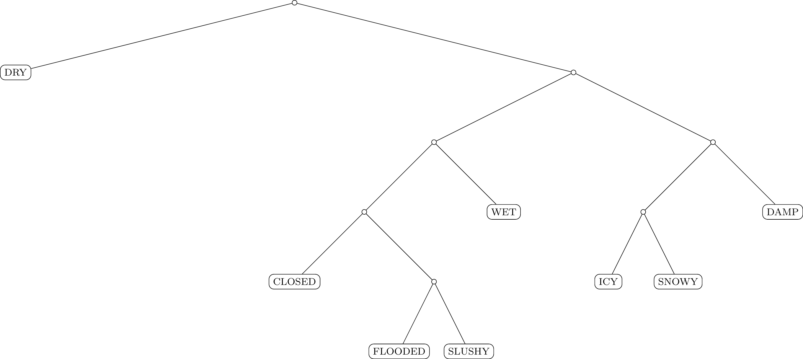
Now, the code for each condition can be determined by tracing the path from the root down to the condition. Each time we take the left branch, we add a 0; each time we take the right branch, we add a 1. For example, based on the tree above,

the code for WET is 101,
the code for SNOWY is 1101,
and so on.