Ns <- 230:260
likelihoods <- sapply(Ns, function(N) {
  if(N >= 241) 1 / prod(N:(N-9))
  else 0
})

plot(Ns, likelihoods, type="h")
$$
$$
In this chapter, we will begin to discuss what makes an estimator good or bad. We will see cases where the MLE is not good and learn strategies for improving upon the MLE.
During World War II, the Allied forces sought to estimate the production of German military equipment, particularly tanks, based on limited data. While intelligence reports provided some information, they were often incomplete or unreliable. Instead, the Allies used information from the German tanks that they captured.
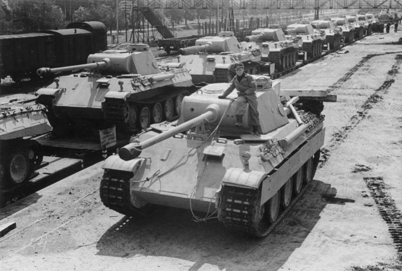
Photo from Bundesarchiv, Bild 183-H26258, distributed under a CC-BY-SA 3.0 DE license
As it turns out, the Germans assigned sequential serial numbers to the tanks that they produced. For simplicity, we will assume that the first tank was assigned a serial number of 1, the second tank was assigned a serial number of 2, and so on. Let’s suppose that 10 tanks from one production line were captured, and they had the following serial numbers:
\[203, 194, 148, 241, 64, 142, 188, 100, 23, 153. \tag{31.1}\]
What should our estimate of \(N\), the total number of tanks be? Let’s use the principle of maximum likelihood. To determine the likelihood \(L(N)\), we need to determine the probability of observing the above sample.
Because Equation 31.2 only decreases as \(N\) increases, we should make \(N\) as small as possible to maximize the likelihood. However, it cannot be any smaller than \(241\) because then the likelihood would be zero. Therefore, the MLE is \(\hat N_{\textrm{MLE}} = 241\). The likelihood is graphed below.
Ns <- 230:260
likelihoods <- sapply(Ns, function(N) {
if(N >= 241) 1 / prod(N:(N-9))
else 0
})
plot(Ns, likelihoods, type="h")
Is \(\hat N_{\textrm{MLE}} = 241\) a good estimate for the number of tanks \(N\) based on the data in Equation 31.1? It is very likely an underestimate, since \(241\) tanks is the minimum number of tanks there could be, based on the observed data. But of course, it could be correct.
It is impossible to evaluate a particular estimate, like \(241\). It is only possible to evaluate the “procedure” for coming up with this estimate, called the estimator. That is, for a sample of \(n\) tanks with serial numbers \[ X_1, X_2, \dots, X_n, \] the maximum likelihood estimator chooses \(N\) to be as small as possible, but no smaller: \[\hat N_{\textrm{MLE}} = \max(X_1, X_2, \dots, X_n). \tag{31.3}\]
The estimator \(\hat N_{\textrm{MLE}}\) is just a random variable, since it depends on the data which is random. To evaluate this estimator, we again turn to probability, continuing the cycle between probability and statistics introduced in Chapter 29.
Let’s apply Definition 31.1 to the MLE Equation 31.3 in the German Tank Problem.
Although the MLE is biased, Equation 31.4 suggests a simple correction that makes the estimator unbiased.
To better understand what it means for an estimator to be unbiased, let’s do a simulation. Suppose that there are \(N = 270\) tanks in the population, and we sample 10 tanks. We simulate the distributions of \(\hat N_{\textrm{MLE}}\) and \(\hat N_{\textrm{MLE}+}\) below.
Notice that \(\hat N_{\textrm{MLE}}\) is never more than \(N = 270\) and severely underestimates on average (\(\text{E}\!\left[ \hat N_{\textrm{MLE}} \right] = \frac{10}{10 + 1} (270 + 1) \approx 246\)). On the other hand, \(\hat N_{\textrm{MLE}+}\) sometimes underestimates and sometimes overestimates, but the estimates average to \(270\).
In Example 30.3, we showed that when we have i.i.d. \(\text{Normal}(\mu, \sigma^2)\) data \(X_1, \dots, X_n\), the maximum likelihood estimator of \(\mu\) (whether or not \(\sigma\) is known) is \[ \hat\mu = \frac{1}{n} \sum_{i=1}^n X_i. \] What is the bias of this estimator for estimating \(\mu\)?
This is a special case of a more general fact: the sample mean is an unbiased estimator of the mean \(\mu = \text{E}\!\left[ X_1 \right]\). The proof is essentially the same.
We now apply Proposition 31.1 to the German Tank Problem.
The strategy of deriving an estimator in Example 31.4 is known as the method of moments. To summarize this method, we start by observing that \(\bar X\) is an unbiased estimator of \[ \text{E}\!\left[ X_1 \right] = h(\theta), \] so if the goal is to estimate \(\theta\), it is reasonable to try \(h^{-1}(\bar X)\). Note that \(h^{-1}(\bar X)\) is not an unbiased estimator in general because \[ \text{E}\!\left[ h^{-1}(\bar X) \right] \neq h^{-1}\Big(\underbrace{\text{E}\!\left[ \bar X \right]}_{h(\theta)} \Big) = \theta, \] unless \(h^{-1}\) is linear (as it was in Example 31.4).
We now have two different unbiased estimators for the number of tanks \(N\):
For the data in Equation 31.1, the two estimators produce very different estimates: \(264.1\) and \(290.2\) tanks, respectively. Which estimate should we trust more? Both estimators are unbiased, so we will need a criterion other than bias. We take up this issue in the next chapter.
Exercise 31.1 (Bias of the Poisson MLE) In Exercise 30.2, you derived the MLE of the parameter \(\mu\) in a \(\text{Poisson}(\mu)\) distribution. What is the bias of this MLE?
Exercise 31.2 (Comparing biased and unbiased estimators of a transformed parameter) Let \(X\) be a single observation from a \(\text{Poisson}(\mu)\) distribution. Suppose that we want to estimate \(\phi = e^{-3\mu}\).
Exercise 31.3 (Estimating a binomial probability) In Example 29.4, we showed that if we roll a skew die \(n\) times and observe \(X\) sixes, the MLE for the probability \(p\) of rolling a six is \[ \hat p = \frac{X}{n}. \] What is the bias of this estimator?
Exercise 31.4 (Another estimator for the German tank problem) In the German tank problem, consider the estimator \[ \hat{N}_{\text{mm}} = \min_i X_i + \max_i X_i. \] Is \(\hat{N}_{\text{mm}}\) biased?
Consider the symmetry of \(\min_i X_i\) and \(\max_i X_i\).
Exercise 31.5 (Estimating variance of a normal distribution with known mean) Let \(X_1, \dots, X_n\) be i.i.d. \(\text{Normal}(\mu, \sigma^2)\), where \(\mu\) is known (but \(\sigma^2\) is not). Find the MLE of \(\sigma^2\). What is its bias?
Exercise 31.6 (Unbiased estimator for the uniform distribution) Let \(X_1, \dots, X_n\) be i.i.d. \(\text{Uniform}(0,\theta)\).
Exercise 31.7 (Randomized response) In surveys, it is sometimes difficult to obtain truthful responses to sensitive questions, such as “Have you ever cheated on an exam?” One way to address this issue is to use the method of randomized response, which allows respondents to answer sensitive questions truthfully while maintaining their privacy.
Here is one way to implement randomized response. Suppose you want to estimate the proportion of students who have cheated on an exam. Each student flips a coin, without showing the result to anyone. If the coin lands heads, then the student answers “yes” (regardless of whether they have ever cheated on an exam). If the coin lands tails, then the student answers the question truthfully. Since only the student knows the outcome of their coin flip, it is impossible to tell whether someone who answered “yes” has actually cheated or not.
Let \(\pi\) be the proportion of students who have cheated. Let \(p\) be the probability that an individual student answers “yes”.
Exercise 31.8 (Estimators of the location parameter in a double exponential distribution) Let \(X_1, X_2, \dots, X_n\) be i.i.d. random variables from a double exponential distribution, with PDF \[ f_\theta(x) = \frac{1}{2} e^{-|x - \theta|}. \]
What is the method of moments estimator of \(\theta\)? Is it unbiased?
Exercise 31.9 (Rayleigh method of moments) In Exercise 30.3, you modeled wind speeds by determining the MLE of \(\sigma^2\) from data.