This chapter introduces two tools for computing probabilities involving conditional probabilities that vastly expand the kinds of problems we can solve.
7.1 Law of Total Probability
In the 2021 NCAA women’s basketball tournament, Stanford defeated South Carolina to advance to the championship, where they would play the winner of the other semifinal between Arizona and UConn. If you were asked at this moment (after Stanford won its semifinal, but before Arizona and UConn’s semifinal) to predict the probability that Stanford will win the championship, how would you calculate it?
Instead of thinking about the probability that Stanford wins the championship directly, we can break down the problem into the probabilities that Stanford beats each possible opponent. Perhaps Stanford matches up well against UConn and has an \(85\%\) chance of winning if their opponent is UConn. But Arizona is a tougher matchup, and Stanford only has a \(60\%\) chance of winning if Arizona advances.
These are both conditional probabilities; the probability that Stanford wins the tournament overall should also account for the probability that Stanford plays each opponent. If UConn is very likely to beat Arizona, then the final probability should be close to \(85\%\). On the other hand, if Arizona is more likely to beat UConn, then the final probability should be closer to \(60\%\).
The Law of Total Probability (LoTP) tells us how to compute the unconditional probability from the conditional ones. It says that we should take a weighted average of the conditional probabilities of Stanford beating a specific opponent, where the weights are the probabilities that Stanford plays each opponent:
To be concrete, suppose that there is a \(90\%\) chance that UConn beats Arizona. Then, the Law of Total Probability says that the probability of Stanford winning is \[ P(\text{Stanford wins}) = 0.90 \cdot 0.85 + 0.10 \cdot 0.60 = 0.825,\] which is very close to the conditional probability that Stanford beats UConn.
On the other hand, if Arizona has a \(75\%\) chance of beating UConn, then the Law of Total Probability says that the probability of Stanford winning is
\[ P(\text{Stanford wins}) = 0.25 \cdot 0.85 + 0.75 \cdot 0.60 = 0.6625,\] which is closer to \(60\%\).
Before we can state the Law of Total Probability, we first need the following definition.
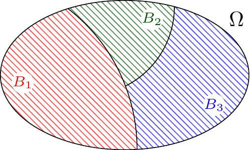
Definition 7.1 (Partition) A partition is a disjoint collection of sets \(B_1, B_2, \dots\) whose union is the sample space \(\Omega\).
That is, for all \(i \neq j\), \[
B_i \cap B_j = \emptyset,
\] and \[
\bigcup_i B_i = \Omega.
\]
Figure 7.1: Three events \(B_1\), \(B_2\), and \(B_3\) that partition the sample space \(\Omega\).
The Law of Total Probability says that if \(B_1, B_2 \dots\) partition the sample space, then the probability \(P(A)\) of any event \(A\) is the weighted average of the conditional probabilities \(P(A \mid B_i)\), where the weights are the probabilities \(P(B_i)\).
Theorem 7.1 (Law of Total Probability) Consider a collection of positive probability events \(B_1, B_2, ...\) that partition the sample space \(\Omega\). Then, for any event \(A\), \[
P(A) = \sum_i P(B_i) P(A \mid B_i)
\tag{7.1}\]
Proof
The sets \(A \cap B_i\) are mutually exclusive, and their union is \(A\). Therefore, by Axiom 3 of Definition 3.1,
\[
P(A) = \sum_i P(A \cap B_i).
\]
But by the multiplication rule (Theorem 5.1), each term inside the sum can be expanded as
\[
P(A \cap B_i) = P(B_i) P(A \mid B_i).
\]
Substituting this into the sum above, we obtain Equation 7.1: \[
P(A) = \sum_i P(B_i) P(A \mid B_i).
\]
In our first example, we use the Law of Total Probability to finally calculate the probability of winning a pass-line bet in craps. It illustrates the most common way the Law of Total Probability is used: to condition on information we wish we knew.
Example 7.1 (Winning a pass-line bet) What is the probability of winning a pass-line bet in craps (Example 1.9)?
If we knew the come-out roll, then we would already be done. In Example 6.6, we calculated the probability of winning a pass-line bet conditional on each possible come-out roll. The following table recalls these values and also gives the unconditional probability of each come-out roll (which can be determined by counting outcomes in Figure 1.9).
\(i\)
\(P(\text{come-out roll is } i)\)
\(P(\text{win} | \text{come-out roll is } i)\)
2
\(\frac{1}{36}\)
\(0\)
3
\(\frac{2}{36}\)
\(0\)
4
\(\frac{3}{36}\)
\(\frac{3}{9}\)
5
\(\frac{4}{36}\)
\(\frac{4}{10}\)
6
\(\frac{5}{36}\)
\(\frac{5}{11}\)
7
\(\frac{6}{36}\)
\(1\)
8
\(\frac{5}{36}\)
\(\frac{5}{11}\)
9
\(\frac{4}{36}\)
\(\frac{4}{10}\)
10
\(\frac{3}{36}\)
\(\frac{3}{9}\)
11
\(\frac{2}{36}\)
\(1\)
12
\(\frac{1}{36}\)
\(0\)
Because the different come-out rolls partition the sample space, we can apply the Law of Total Probability: \[ P(\text{win}) = \sum_{i=2}^{12} P(\text{come-out roll is } i) P(\text{win} \mid \text{come-out roll is } i). \]
Somewhat magically, the Law of Total Probability allows us to condition on the come-out roll (what we wish we knew) despite us not yet knowing what it is!
This sum has several terms and is most easily evaluated by a computer.
The probability is about \(49.29\%\). Therefore, the casino has a small but definite edge!
In the next example we compute the probability that a COVID-19 antigen test gives the correct reading. Again, the Law of Total Probability allows us to condition on what we wish we knew, which in this case is whether or not the person is infected.
Example 7.2 (Probability that COVID-19 antigen test is correct) Recall Example 6.9 where we imagined having a random New York City (NYC) resident take two COVID-19 antigen tests at the end of March 2020. What is the probability that the first test gives the correct reading?
We will use the notation introduced in Example 6.9. Usually, the accuracy of the test is discussed in terms of false positive and false negative rates:
False positive rate: If a person is not infected with COVID-19, then the test comes back positive \(1\%\) of the time, so \(P(T_1|I^c) = 0.01\). By the complement rule (Proposition 4.1), we also have \(P(T_1^c \mid I^c) = 0.99\).
False negative rate: If a person is infected with COVID-19, then the test will come back negative \(20\%\) of the time, so \(P(T_1^c \mid I ) = 0.20\). By the complement rule (Proposition 4.1), we also have \(P(T_1 \mid I) = 0.80\).
Based on historical NYC population data and the number of confirmed COVID-19 cases at the time, it is reasonable to think that the probability of a random person being infected is roughly \(P(I) = 0.0005\). By the complement rule, the probability of a random person not being infected is \(P(I^c) = 0.9995\).
To compute the probability that the test has the correct reading, we condition on what we wish we knew: whether or not the person is infected with COVID-19.
Overall, the accuracy of the COVID-19 antigen test is very high for a random person. But this is only because it is very accurate when someone doesn’t have COVID-19, and most people do not have COVID-19!
The Law of Total Probability also comes in handy when we analyze a random process that can repeat itself or start over. By conditioning on different events that might occur before it restarts, we can obtain a recursive formula that allows us to calculate a probability of interest.
Example 7.3 (Branching Process) Amoebas are single-celled organisms that reproduce asexually by splitting into two cells in a process called binary fission. One common model in biology for an amoeba population is a branching process. In a branching process, each amoeba can die, stay alive, or split into two at each time point (e.g., every minute), independently of the other amoebas and everything that happened previously.
Consider a population consisting of a single amoeba. Suppose furthermore that each amoeba is equally likely to die, stay alive, or split into two. What is the probability that this amoeba population eventually goes extinct?
We will use \(p = P(E)\) to denote the probability of the event \(E\) that the population goes extinct. After one minute, one of three events could have transpired:
\(D\): The initial amoeba dies and the population has died out.
\(L\): The initial amoeba survives and the process starts over.
\(S\): The initial amoeba splits into two children, and now two new versions of the process start from the beginning.
Because these three events partition the sample space, we can apply the Law of Total Probability in hopes of getting an expression for \(p\) in terms of itself:
\[
\begin{align*}
p &= P(E)\\
&= P(D)P(E \mid D) + P(L)P(E \mid L) + P(S)P(E \mid S) & \text{(LoTP)}\\
&= \frac{1}{3}P(E \mid D) + \frac{1}{3}P(E \mid L) + \frac{1}{3}P(E \mid S) & \text{(plug-in probabilities)}\\
\end{align*}
\] We examine each one of these conditional probabilities separately:
\(P(E \mid D)\): If the initial amoeba dies in the first minute, then the population has gone extinct. This conditional probability is \(1\).
\(P(E \mid L)\): If the initial amoeba lives, then the process restarts. Because the first amoeba behaves independently of its previous self, there is no difference between this process and the original process, so the conditional probability that the whole population goes extinct should still be \(p\).
\(P(E \mid S)\): When the initial amoeba splits into two children, we now have two new versions of the process that start from the beginning. Let \(E_1\) be the event that the first child’s lineage dies out and \(E_2\) be the event that the second child’s lineage dies out. Conditional on \(S\), the population goes extinct if and only if both lineages die out. Also conditional on \(S\), the two children behave independently of each other (as will their children, and so on), so their extinctions are conditionally independent events given \(S\). Therefore, \[
\begin{align*}
P(E \mid S) &= P(E_1 \cap E_2 \mid S) & \text{(same event conditional on } S \text{)}\\
&= P(E_1 \mid S)P(E_2 \mid S) & \text{(conditional independence)}\\
&= p^2. & \text{(same reasoning as } P(E \mid L) \text{)}
\end{align*}
\]
Substituting these values back into our earlier Law of Total Probability computation, we find that \[p = \frac{1}{3} + \frac{1}{3}p + \frac{1}{3}p^2,\] so the solution \(p\) must satisfy the quadratic equation \[\frac{1}{3}p^2 - \frac{2}{3}p + \frac{1}{3} = 0,\] which has only one solution: \(p=1\). This amoeba population will eventually go extinct!
Note on formally computing \(P(E \mid L)\)
Our computation of \(P(E \mid L)\) (and therefore also \(P(E \mid S)\)) is a little more informal than usual. We did not apply the definition of conditional probability (Definition 5.1) like we typically do, and instead said that \(P(E \mid L)\) should equal \(P(E)\) based on intuitive arguments. In such recursive problems, justifying things more formally is tricky and beyond the scope of this book. Arguments like the one we presented are sufficient for our purposes, and they will get you the right answer!
The Law of Total Probability provides insight into Simpson’s paradox, a paradox where a trend that appears in multiple sub-populations disappears (or even reverses) when aggregated over the entire population. It is named for British statistician Edward H. Simpson, who was recruited to Bletchley Park during World War II to work on codebreaking. During his time there, he developed an interest in statistics, and after the war, he pursued a Ph.D. in mathematical statistics at Cambridge. It was there that he wrote the paper (Simpson 1951) that introduced his namesake paradox. He is also the namesake of the Simpson index (Simpson 1949), which is used in ecology to measure biodiversity, which you can explore in Exercise 7.5.
Edward H. Simpson (1922-2019)
Example 7.4 (Simpson’s paradox and the death penalty)Radelet and Pierce (1991) examined the effect of race on the probability of receiving the death penalty for homicide convictions in Florida.
Table 7.1 shows data from defendants who were convicted of multiple homicides in Florida between 1976 and 1987.
Table 7.1: Death penalty rate by race of the defendant. The higher rate is highlighted in red, and the higher number of defendants is underlined.
Black
White
# Defendants
% Death Penalty
# Defendants
% Death Penalty
\(191\)
\(7.9\%\)
\(\underline{483}\)
\(\textcolor{red}{11.0\%}\)
At first glance, it appears that white defendants received the death penalty at a higher rate. Is that the end of the story? Table 7.2, which breaks the data down by the race of the victims, tells a different story.
Table 7.2: Death penalty rate by race of the defendant and race of the homicide victims. The higher rate in each row is highlighted in red, and the higher number of defendants is underlined.
Black Defendant
White Defendant
# Defendants
% Death Penalty
# Defendants
% Death Penalty
Black Victims
\(\underline{143}\)
\(\textcolor{red}{2.8\%}\)
\(16\)
\(0.0\%\)
White Victims
\(48\)
\(\textcolor{red}{22.9\%}\)
\(\underline{467}\)
\(11.3\%\)
Total
\(191\)
\(7.9\%\)
\(\underline{483}\)
\(\textcolor{red}{11.0\%}\)
Black defendants have a higher death penalty rate, regardless of the race of their victims, yet their overall death penalty rate is lower! What explains this apparent contradiction?
Black defendants appear to be sentenced to death at a slightly higher rate than white defendants, but the race of the victim seems to play a bigger role; multiple homicides involving white victims are much more likely to result in the death penalty. Because most homicide is intraracial (the victim is the same race as the perpetrator), white defendants have a higher death penalty rate overall—because their victims are more likely to be white.
The Law of Total Probability helps explain this effect. Consider a randomly selected defendant. We will analyze the probability that they receive the death penalty by race.
First, consider the conditional probability function \(\widetilde{P}_{\text{B}}(\cdot) \overset{\text{def}}{=}P( \cdot \mid \text{Black defendant})\). These conditional probabilities can be determined from the first two columns of Table 7.2. \[\begin{align*}
P&(\text{Death} \mid \text{Black defendant}) \\
&= \widetilde{P}_{\text{B}}(\text{Death} ) & \text{(Definition of $\widetilde{P}$)}\\
&=\widetilde{P}_{\text{B}}(\text{Black victim})\widetilde{P}_{\text{B}}(\text{Death} \mid \text{Black victim} ) & \\
& \quad + \widetilde{P}_{\text{B}}(\text{White victim})\widetilde{P}_{\text{B}}(\text{Death} \mid \text{White victim} ) & \text{(Law of Total Probability)} \\
&= \frac{143}{191} \cdot 0.028 + \frac{48}{191} \cdot 0.229 & \\
&\approx 0.079.
\end{align*}\]
The overall death penalty rate is a weighted average of \(0.028\) and \(0.229\), with more weight on the lower number.
Next, consider the conditional probability function \(\widetilde{P}_{\text{W}}(\cdot) \overset{\text{def}}{=}P( \cdot \mid \text{White defendant})\). These conditional probabilities can be determined from the last two columns of Table 7.2.
Here, the overall death penalty rate is a weighted average of \(0\) and \(0.113\), with more weight on the higher number. Because the weights are different, it is actually possible for \[
\widetilde{P}_{\text{W}}(\text{Death} ) > \widetilde{P}_{\text{B}}(\text{Death} ),
\] even though they are just a weighted average of \[
\widetilde{P}_{\text{W}}(\text{Death} \mid \text{Black victim} ) < \widetilde{P}_{\text{B}}(\text{Death} \mid \text{Black victim} )
\] and \[
\widetilde{P}_{\text{W}}(\text{Death} \mid \text{White victim} ) < \widetilde{P}_{\text{B}}(\text{Death} \mid \text{White victim} ).
\] This reversal of apparent trends when subpopulations are aggregated is the essence of Simpson’s paradox.
Simpson’s paradox teaches us that looking at aggregate data can be misleading. However, there are situations where this reversal cannot occur. Exercise 7.6 asks you to examine two situations where Simpson’s paradox cannot occur.
7.2 Bayes’ Rule
During the COVID-19 pandemic, identifying who was and was not infected was critical to slowing the spread of the virus. This was especially true in New York City in March 2020, when hospitals were overwhelmed with COVID-19 patients. Yet city policy at the time limited testing to symptomatic individuals. As we saw in Example 7.2, however, the COVID-19 antigen test has high overall accuracy. So why not test everyone?
To understand this policy, imagine that a random NYC resident takes the test, and it comes back positive. We saw in Example 7.2 that \[
P(T_1 \mid I)
\] is high. However, what we really want to know is \[
P(I \mid T_1),
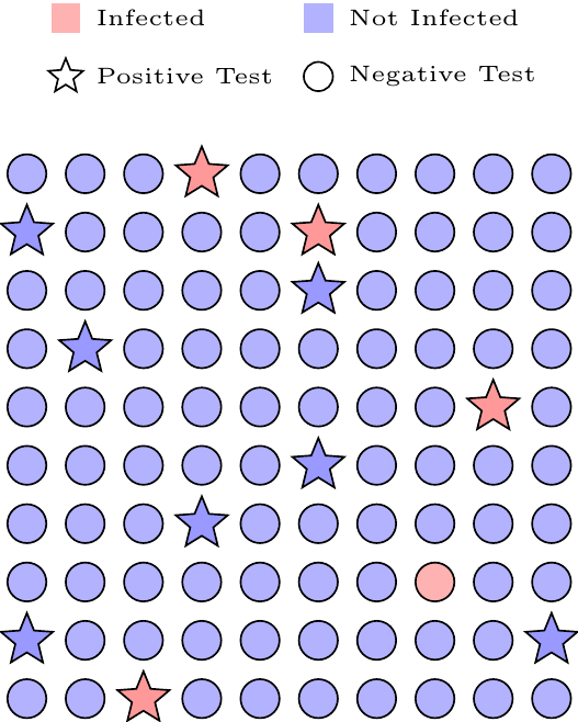
\] the probability that they are infected given this information. These two probabilities are not the same, and in fact they can be quite different, as Figure 7.2 illustrates.
Figure 7.2: Visual depiction of \(100\) NYC residents. Red and blue indicate infected and uninfected, respectively, while stars and circles indicate positive tests and negative tests, respectively.
In Figure 7.2, the probability of a positive test given infection is high (most red shapes are stars), yet the probability of infection given a positive test is low (most stars are blue). This is because, although it is unlikely for uninfected people to get a positive test, there are so many more uninfected people that most of the positive tests come from these unlikely mistakes. Essentially, if NYC had suggested that every resident take tests, then most of the positive tests would have been false positives, causing unnecessary stress and panic. By restricting the tests to symptomatic people only, who are more likely to be infected than the general population, NYC avoided this issue.
Bayes’ rule, which we describe below, is a computational tool that enables us to properly handle situations like this one. In particular, Bayes’ rule enables us to use \(P(A \mid B)\) to compute the reverse conditional probability \(P(B \mid A)\).
Theorem 7.2 (Bayes’ rule) Let \(A\) and \(B\) be events with positive probabilities. Then: \[ P(B \mid A) = \frac{P(B) P(A \mid B)}{P(A)}. \tag{7.2}\]
In many cases, we do not know \(P(A)\) and need to calculate it using the Law of Total Probability (Theorem 7.1), in which case Equation 7.2 becomes:
\[
P(B \mid A) = \frac{P(B) P(A \mid B)}{P(B) P(A \mid B) + P(B^c) P(A \mid B^c)}.
\tag{7.3}\]
Proof
Bayes’ rule follows immediately from the two different ways of expanding \(P(A \cap B)\) using the multiplication rule (Corollary 5.1):
\[
P(B) P(A \mid B) = P(A) P(B \mid A).
\]
Now, divide both sides by \(P(A)\) to obtain Equation 7.2.
We can use Bayes’ rule to calculate the probability that a random NYC resident who tested positive is actually infected.
Example 7.5 (Positive COVID-19 test) In Example 6.9, we considered a randomly selected person from New York City (NYC) taking a COVID-19 antigen test in March 2020. If this test comes back positive, what’s the probability that they have COVID-19?
Again, we use the notation from Example 6.9. In Example 7.2, we supposed that the false negative rate was \[
P(T_1^c \mid I) = 0.20
\] and the false positive rate was \[
P(T_1 \mid I^c) = 0.01.
\]
From this, we can use the complement rule to conclude that \(P(T_1 \mid I) = 1 - 0.20 = 0.80\). Since we know \(P(T_1 \mid I)\), but want to know \(P(I \mid T_1)\), we should use Bayes’ rule. Since we do not know the denominator, \(P(T_1)\), we need the expanded version of Bayes’ rule (Equation 7.3):
\[
\begin{align*}
P( \mid T_1) &= \frac{P(I) P(T_1 \mid I)}{P(I) P(T_1 \mid I) + P(I^c) P(T_1 \mid I^c)}
& \text{(Bayes' rule)}\\
&= \frac{0.0005 \cdot 0.80}{0.0005 \cdot 0.80 + 0.9995 \cdot 0.01} & \text{(plug in probabilities)}\\
&\approx 0.03848 & \text{(simplify)}
\end{align*}
\] There is less than a \(4\%\) chance that the person actually has COVID-19, even though they just tested positive!
When it comes to medical diagnoses, it is a good idea to always seek a second opinion. What if the person from Example 7.5 has their second COVID-19 antigen test also come back positive?
Example 7.6 (Two positive COVID-19 tests) If the random NYC resident from Example 7.5 has their second COVID-19 antigen test come back positive as well, what is the probability now that they are infected?
Again we use the events from Example 6.9 and, as Example 6.9 justifies, we will assume that \(T_1\) and \(T_2\) are conditionally independent given \(I\) and \(I^c\).
First, we calculate \(P(I \mid T_1, T_2)\) directly using the expanded version of Bayes’ rule (Equation 7.3).
A second test helps a lot! Now, the person knows that they are quite likely to have COVID.
We also discuss another way to approach this problem. In Example 7.5, we updated the probability of infection from \(P(I) = 0.0005\) to \(P(I \mid T_1) \approx 0.03848\) after the first positive test. We can use \(0.03848\) as the new “prior” probability of infection in Bayes’ rule to calculate \(P(I \mid T_1, T_2)\).
Indeed, we can apply Bayes’ rule to the conditional probability function \(P(\cdot \mid T_1)\) to obtain the same answer:
Whether we apply Bayes’ rule once using the combined result of two positive tests, or apply it sequentially, updating the probability after each test, we arrive at the same final probability. This demonstrates the logical consistency of Bayes’ rule as a method for updating probabilities in light of new evidence.
As the person takes more tests, the probability of infection can continue to be updated in the same way, by applying Bayes’ rule after each test. The code snippet below allows you to get a feel for how this probability changes as a function of:
the prior probability \(P(I)\) of the person being infected,
the false positive rate \(P(T_1 \mid I^c)\),
the false negative rate \(P(T_1^c \mid I)\), and
the number of positive test results.
Our next example illustrates how Bayes’ rule can be used to build a spam filter. While naive Bayes is a relatively old approach for spam filtering, Bayes’ rule remains central to modern classification systems in artificial intelligence.
Example 7.7 (Detecting spam with a naive Bayes classifier) Suppose we are building a classifier that labels emails as either spam or not spam (also called “ham”). A common approach is to use a naive Bayes classifier. Once given the contents of an email, a naive Bayes classifier uses Bayes’ rule to compute the probability that it is spam.
As an example, consider an email consisting of the single sentence: \[
\text{``win free money!''}
\]
This email obviously looks suspicious; words like \(\text{``win"}\), \(\text{``free"}\), and \(\text{``money"}\) tend to appear more often in spam emails. If we had a labeled dataset of spam and ham emails, we could use it to estimate the probability of each word appearing in either a spam or ham email:
We can also use the proportion of spam and ham emails in the dataset to estimate the probability that a random email is spam or ham: \[
P(\text{spam}) = 0.1 \quad \text{and} \quad P(\text{ham}) = 0.9.
\]
To compute the probability that the above email is spam (or ham), we apply Bayes’ rule (Theorem 7.2):
The naive Bayes assumption is that the words in the email are conditionally independent given the label of the email. That is, once we know the email is spam (or ham), we treat the words as independent:
We could also compute the denominator under the naive Bayes assumption, but it is not necessary. What matters is the ratio of the two probabilities, and the shared denominator cancels out: \[
\frac{P(\text{spam} \mid \text{``win free money!''})}{P(\text{ham} \mid \text{``win free money!''})}
= \frac{P(\text{spam}) P(\text{``win''} \mid \text{spam}) P(\text{``free''} \mid \text{spam}) P(\text{``money''} \mid \text{spam})}
{P(\text{ham}) P(\text{``win''} \mid \text{ham}) P(\text{``free''} \mid \text{ham}) P(\text{``money''} \mid \text{ham})}.
\]
Substituting in the values above we find that \[
\frac{P(\text{spam} \mid \text{``win free money!''})}{P(\text{ham} \mid \text{``win free money!''})} = \frac{0.1 \cdot 0.02 \cdot 0.05 \cdot 0.1}{0.9 \cdot 0.0005 \cdot 0.001 \cdot 0.01} \approx 2222.22.
\]
So the classifier believes the email is more than 2000 times more likely to be spam than ham, so this email is sent to the spam folder.
Is the naive Bayes assumption reasonable?
The naive Bayes assumption is called naive because—well—it is! In reality, words are not independent given the label of the email. Still, this assumption often works surprisingly well.
Why is the assumption reasonable, even when we know that it is not true? When we do not know the label of the email, words are highly dependent. Words like \(\text{``money''}\) make an email more likely to be spam, and spam emails are more likely to contain related words like \(\text{``win''}\) and \(\text{``free''}\). Once we know that the email is spam, however, seeing \(\text{``money''}\) informs us much less about the remaining words. Because we already know that the email is spam, we already know that words like \(\text{``win''}\) and \(\text{``free''}\) are likely to appear. This is why the naive Bayes assumption, although not perfect, is reasonable.
7.3 Exercises
Exercise 7.1 (Two spades) If we draw two cards from a standard shuffled deck of \(52\) playing cards, what is the probability that the second card is a spade? Explain how you could have arrived at this answer using symmetry.
Exercise 7.2 (Probability of the second draft pick) Recalling the NBA draft lottery from Example 5.3, what is the probability that the Hornets get the second pick? Is it possible to calculate this probability using symmetry?
Exercise 7.3 (The rainy dinner party) You are hosting a dinner party tomorrow and your friend tells you that there is a \(90\%\) chance that they will show up if it does not rain, but only a \(50\%\) chance if it does. If the forecast predicts a \(10\%\) chance of rain tomorrow, what is the probability that your friend will come to the dinner party?
Exercise 7.4 (Crapless craps) One variant of craps in casinos is “crapless craps.” In crapless craps, any come-out roll (except seven) can become the point. That is, the shooter no longer loses on the come-out roll by rolling a two, three, or twelve; that number simply becomes the point, and a pass-line bet wins if the shooter rolls the point again before rolling a seven. Likewise, the shooter no longer wins on the come-out roll by rolling an eleven; eleven simply becomes the point.
Calculate the probability of winning a pass-line bet in crapless craps, and compare it to the probability of winning in regular craps.
Exercise 7.5 (Simpson index) The Simpson index (named for Edward H. Simpson, also the namesake of Simpson’s paradox) is widely used in ecology to measure biodiversity. If a community contains \(K\) species, with proportions \[
p_1, p_2, \dots, p_K,
\] the Simpson diversity index is defined as the probability that two randomly chosen individuals from the community belong to different species.
Express the Simpson diversity index in terms of \(p_1, p_2, \dots, p_K\). Assume that the individuals are chosen with replacement (i.e., independently).
Exercise 7.6 (When Simpson’s paradox is impossible) Consider Example 7.4, where we saw that \[
\begin{align}
\widetilde{P}_{\text{W}}(\text{Death} \mid \text{Black victim} ) &< \widetilde{P}_{\text{B}}(\text{Death} \mid \text{Black victim} ) \\
\widetilde{P}_{\text{W}}(\text{Death} \mid \text{White victim} ) &< \widetilde{P}_{\text{B}}(\text{Death} \mid \text{White victim} ).
\end{align}
\tag{7.4}\]
Simpson’s paradox says that despite Equation 7.4, it is nevertheless possible for \[
\widetilde{P}_{\text{W}}(\text{Death} ) > \widetilde{P}_{\text{B}}(\text{Death} ).
\]
In this exercise, you will explore two situations where it is impossible for this reversal to happen. That is, the two conditions in Equation 7.4 also imply \[
\widetilde{P}_{\text{W}}(\text{Death} ) < \widetilde{P}_{\text{B}}(\text{Death} ).
\]
Show that Simpson’s paradox would not be possible if there were no relationship between the race of the defendant and the race of the victim. That is, \[
P(\text{White victim} \mid \text{Black defendant}) = P(\text{White victim} \mid \text{White defendant}).
\]
Show that Simpson’s paradox would not be possible if \[
\widetilde{P}_{\text{W}}(\text{Death} \mid \text{White victim} ) < \widetilde{P}_{\text{B}}(\text{Death} \mid \text{Black victim} ).
\]
Exercise 7.7 (Two spades and Bayes’ rule) If we draw two cards from a standard shuffled deck of \(52\) playing cards, what is the probability that the second card is a spade given that the first card was a spade? What about the probability that the first card is a spade given that the second card is a spade?
Exercise 7.8 (COVID-19 vaccines) At one point during the pandemic, it was reported that \(75\%\) of the people who had an active COVID infection had received the vaccine. Does this mean that the vaccine is ineffective? Supposing that \(x \%\) of the population is vaccinated, for what values of \(x\) would you be concerned that the vaccine is working versus not working?
Exercise 7.9 (Billionaire’s goat) You are on a game show with three doors. Behind one door is a car, and behind the other two are goats. One of the goats belongs to a billionaire, and the billionaire is willing to pay a handsome sum (much more than the car is worth) to get their goat back. You can tell the billionaire’s goat apart from the regular goat because it has a gold collar around its neck.
You choose Door 1. The host, who knows there is a car behind one door and goats behind the other two, opens Door 3 to reveal a goat, but it is not the billionaire’s goat.
You now have the choice: stick with Door 1 or switch to Door 2. What is the probability that the billionaire’s goat is behind Door 1? What is the probability it’s behind Door 2? Should you switch?
Radelet, Michael L, and Glenn L Pierce. 1991. “Choosing Those Who Will Die: Race and the Death Penalty in Florida.”Fla. L. Rev. 43: 1.
Simpson, Edward H. 1949. “Measurement of Diversity.”Nature 163 (4148): 688–88.
———. 1951. “The Interpretation of Interaction in Contingency Tables.”Journal of the Royal Statistical Society: Series B (Methodological) 13 (2): 238–41.