41 General Order Statistics

In Chapter 40, we examined the distribution of the smallest (minimum) and largest (maximum) of $n$ i.i.d. random variables. In this chapter, we will examine the distribution of the $k$th smallest.

Definition 41.1 Let $X_1, \dots, X_n$ be random variables. Then, $X_{(k)}$ denotes the $k$th smallest number and is called the $k$th order statistic.

That is, \[\begin{align} X_{(1)} &= \min(X_1, \dots, X_n) \\ X_{(2)} &= \text{2nd smallest number} \\ &\vdots \\ X_{\left( \frac{n+1}{2} \right)} &= \text{median}(X_1, \dots, X_n) & \text{when $n$ is odd} \\ &\vdots \\ X_{(n-1)} &= \text{2nd largest number} \\ X_{(n)} &= \max(X_1, \dots, X_n) \end{align}\]

For example, if we observe \[ X_1 = 0.87, X_2 = 1.34, X_3 = 0.22, X_4 = 0.36, \] then the order statistics are \[ X_{(1)} = 0.22, X_{(2)} = 0.36, X_{(3)} = 0.87, X_{(4)} = 1.34. \]

Throughout this chapter, we will restrict our attention to order statistics of i.i.d. continuous random variables. The theory for discrete random variables is much more difficult because of the positive probability of ties.

41.1 Distribution of Order Statistics

Proposition 41.1 (Distribution of order statistics) Let $X_1, \dots, X_n$ be i.i.d. continuous random variables with PDF $f(x)$ and CDF $F(x)$. Then, the PDF of the $k$th order statistic, $X_{(k)}$, is \[ f_{X_{(k)}}(t) = n \binom{n-1}{k-1} F(t)^{k-1} f(t) (1 - F(t))^{n-k}. \tag{41.1}\]

Rigorous Proof

By the probability integral transform (Theorem 20.1) $U_i = F(X_i)$ follows a standard uniform distribution, and since $F$ is monotone, $U_{(k)} = F(X_{(k)})$. So we can derive the PDF of $U_{(k)}$ and transform it to obtain the PDF of $X_{(k)}$. First, we determine the CDF of $U_{(k)}$. In order for $\{ U_{(k)} \leq t \}$, $k$ or more of $U_1, \dots, U_n$ must be $\leq t$. That is, \[ F_{U_{(k)}}(t) = \sum_{j=k}^n \binom{n}{j} t^j (1 - t)^{n-j}. \] Now, we take the derivative to obtain the PDF of $U_{(k)}$. \[\begin{alignat*}{2} f_{U_{(k)}}(t) &= F'_{U_{(k)}}(t) \\ &= \sum_{j=k}^n j\binom{n}{j} t^{j-1} (1 - t)^{n-j} - \sum_{j=k}^{n-1} (n-j)\binom{n}{j} t^j (1 - t)^{n - j - 1} && (\text{$j=n$ term in second sum is zero})\\ &= \sum_{j=k}^n n\binom{n-1}{j-1} t^{j-1} (1 - t)^{n-j} - \sum_{j=k}^{n-1} n\binom{n-1}{j} t^j (1 - t)^{n - j - 1} \qquad \qquad && (\text{``choosing a captain'' identity}) \\ &= \sum_{j=k}^n n\binom{n-1}{j-1} t^{j-1} (1 - t)^{n-j} - \sum_{j'=k+1}^{n} n\binom{n-1}{j'-1} t^{j'-1} (1 - t)^{n - j'} && (j' = j+1) \end{alignat*}\] Now, the second sum cancels all terms in the first sum, except for the first term, leaving us with \[ f_{U_{(k)}}(t) = n\binom{n-1}{k-1} t^{k-1} (1 - t)^{n-k}. \] Now, for the general case, the CDF is \[ F_{X_{(k)}}(t) = P(X_{(k)} \leq t) = P(F^{-1}(U_{(k)}) \leq t) = P(U_{(k)} \leq F(t)) = F_{U_{(k)}}(F(t)). \] Therefore, the PDF is \[\begin{align} f_{X_{(k)}}(t) = F'_{X_{(k)}}(t) &= f_{U_{(k)}}(F(t)) f(t) \\ &= n\binom{n-1}{k-1} F(t)^{k-1} (1 - F(t))^{n-k} f(t). \end{align}\]

Heuristic Proof

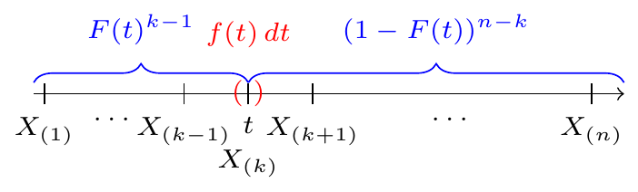
Figure 41.1: Schematic for the PDF of $X_{(k)}$ at $t$.

In order for $X_{(k)}$ to be near $t$, we need $k-1$ of the $X_i$s to be to the left of $t$ and $n-k$ of the $X_i$s to be to the right. In all, there are \[ \frac{n!}{(k-1)!1!(n-k)!} = n \binom{n-1}{k-1} \] ways to arrange $X_1, \dots, X_n$ so that the $k$th smallest is near $t$. Then:

Each of the $k-1$ smallest random variables has probability $P(X_i < t) = F(t)$ of being to the left of $t$.
Each of the $n-k$ largest random variables has probability $P(X_i > t) = 1 - F(t)$ of being to the right of $t$.
The $k$th smallest observation has probability $f(t) \, \Delta t$ of being near $t$.

Hence, the probability that $X_{(k)}$ is near $t$ is \[\begin{align*} f_{X_{(k)}}(t) \,\Delta t &\approx P\left( t - \frac{\Delta t}{2} \leq X_{(k)} \leq t + \frac{\Delta t}{2} \right) \\ &\approx n \binom{n-1}{k-1} F(t)^{k-1} (1 - F(t))^{n-k} f(t) \, \Delta t. \end{align*}\] Dividing both sides by $\Delta t$, we obtain Equation 41.1.

Check that when we set $k = 1$ or $k = n$ in Equation 41.1, we recover the PDF of the minimum and maximum from Chapter 40.

Next, we apply Proposition 41.1 to the median.

Example 41.1 (Estimating the median of the exponential distribution) In Example 19.4, we showed that the median of an $\text{Exponential}(\lambda)$ random variable is $-\frac{\log(.5)}{\lambda}$.

If we wanted to estimate this median, there are two natural options:

We could estimate $\lambda$ and plug this estimate into the above function. That is, $-\log(.5) \bar X$.
We could estimate the median by the sample median $X_{\left(\frac{n+1}{2}\right)}$ (at least when $n$ is odd).

Which estimator is better?

The first estimator is a linear transformation of the sample mean, so we can easily calculate its expectation and variance: \[\begin{align} \text{E}\!\left[ -\log(.5)\bar X \right] &= -\log(.5) \text{E}\!\left[ \bar X \right] = -\frac{\log(.5)}{\lambda} \\ \text{Var}\!\left[ -\log(.5)\bar X \right] &= \log(.5)^2 \text{Var}\!\left[ \bar X \right] = \frac{\log(.5)^2}{n\lambda^2}. \end{align}\] We see that $-\log(.5)\bar X$ is unbiased with \[ \text{MSE}\!\left[ -\log(.5)\bar X \right] = \frac{\log(.5)^2}{n\lambda^2}. \tag{41.2}\]

The second estimator is an order statistic. To determine its expectation and variance, we will first need to determine its distribution. To make things simpler, we note that each $X_i$ can be represented as a scale transformation of a standard exponential, $X_i = \frac{1}{\lambda} Z_i$, so \[X_{\left(\frac{n+1}{2}\right)} = \frac{1}{\lambda} Z_{\left(\frac{n+1}{2}\right)}.\] So we just need to determine the distribution of the order statistics of i.i.d. $\textrm{Exponential}(\lambda=1)$ random variables.

By Proposition 41.1, $Z_{\left(\frac{n+1}{2}\right)}$ has PDF \[ \begin{align} f_{Z_{\left(\frac{n+1}{2}\right)}}(t) &= n \binom{n-1}{(n-1)/2} F(t)^{(n-1)/2} f(t) (1 - F(t))^{(n-1)/2} \\ &= n \binom{n-1}{(n-1)/2} (1 - e^{-t})^{(n-1)/2} e^{-t} (e^{-t})^{(n-1)/2}. \end{align} \]

This PDF is not easy to integrate by hand, so we will use R to integrate it numerically for a particular value of $n$. When $n=9$, the first two moments of the median $Z_{\left(\frac{n+1}{2}\right)} = Z_{(5)}$ are calculated below. The PDF of $Z_{(5)}$ is also graphed along with the PDF of each individual observation $Z_1$.

so the expectation and variance are \[\begin{align} \text{E}\!\left[ Z_{(5)} \right] &\approx 0.7456 \\ \text{Var}\!\left[ Z_{(5)} \right] &= \text{E}\!\left[ Z_{(5)}^2 \right] - \text{E}\!\left[ Z_{(5)} \right]^2 \approx 0.6721 - (0.7456)^2 \approx 0.1162. \end{align}\]

Therefore, the bias, variance, and MSE of the median $X_{(5)}$ when $n=9$ are: \[\begin{align} \text{E}\!\left[ X_{(5)} \right] - \frac{-\log(.5)}{\lambda} &= \text{E}\!\left[ \frac{1}{\lambda} Z_{(5)} \right] - \frac{-\log(.5)}{\lambda} \\ &= \frac{0.7456 + \log(.5)}{\lambda} \approx \frac{0.0525}{\lambda} \\ \text{Var}\!\left[ X_{(5)} \right] &= \text{Var}\!\left[ \frac{1}{\lambda} Z_{(5)} \right] \approx \frac{0.1162}{\lambda^2} \\ \text{MSE}\!\left[ X_{(5)} \right] &\approx \left(\frac{0.0525}{\lambda}\right)^2 + \frac{0.1162}{\lambda^2} = \frac{0.1189}{\lambda^2}. \end{align}\]

Comparing this with Equation 41.2 for $n = 9$, this estimator has a larger MSE, so the first estimator was better.

In the example above, we numerically approximated the MSE of the median of a random sample of size $n=9$ from an $\text{Exponential}(\lambda)$ distribution. The disadvantages of numerical approximation are:

It is not exact.
We have to separately calculate the MSE for each value of $n$.

There is a way to calculate the exact MSE as a function of $n$, by applying the memoryless property of the exponential distribution. The details are in Exercise 41.5.

Other order statistics besides the median, minimum, and maximum can be useful.

Example 41.2 (Interquartile range) If we observe $X_1, \dots, X_n$, what is the best way to visualize the data? One way is using a boxplot.

A boxplot displays five order statistics: the minimum, the first quartile, the median, the third quartile, and the maximum. The width of the “box” is the distance between the first and third quartiles, called the interquartile range.

How large is the interquartile range if $X_1, \dots, X_n$ are i.i.d. $\textrm{Uniform}(a= 0, b= 1)$? To be concrete, suppose $n = 9$ so that the first and third quartiles are $X_{(3)}$ and $X_{(7)}$, respectively, and the interquartile range is $X_{(7)} - X_{(3)}$.

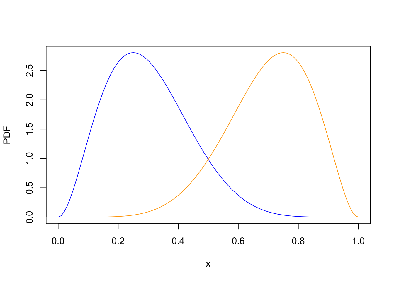
To calculate $\text{E}\!\left[ X_{(7)} - X_{(3)} \right]$, we need the distributions of $X_{(3)}$ and $X_{(7)}$. By Proposition 41.1, the PDF of the $k$th order statistic of $n=9$ i.i.d. standard uniform random variables is \[ f_{X_{(k)}}(t) = 9\binom{8}{k-1} t^{k-1} (1 - t)^{9 - k}. \tag{41.3}\]

The distributions of $\textcolor{blue}{X_{(3)}}$ and $\textcolor{orange}{X_{(7)}}$. As expected, the first quartile has most of its mass near $0.25$, while the third quartile has most of its mass near $0.75$.

To calculate their exact expected values, we integrate: \[\begin{align} \text{E}\!\left[ X_{(k)} \right] &= \int_0^1 t \cdot 9\binom{8}{k-1} t^{k-1} (1 - t)^{9-k}\,dt \\ &= 9\binom{8}{k-1} \int_0^1 t^k (1 - t)^{9-k} \,dt \\ &= \frac{9\binom{8}{k-1}}{10 \binom{9}{k}} \underbrace{\int_0^1 10 \binom{9}{(k+1)-1} t^{(k+1)-1} (1 - t)^{10-(k+1)} \,dt}_{1} \\ &= \frac{k}{10}. \end{align}\] In the second-to-last line, we recognized the integrand as a PDF of the form Equation 41.1 (with $10$ and $k+1$ for $n$ and $k$, respectively). Since it is a PDF, it must integrate to $1$.

Therefore, the expected interquartile range is \[ \text{E}\!\left[ X_{(7)} - X_{(3)} \right] = \text{E}\!\left[ X_{(7)} \right] - \text{E}\!\left[ X_{(3)} \right] = \frac{7}{10} - \frac{3}{10} = 0.4. \]

Note that the true interquartile range for the standard uniform distribution is \[ F^{-1}(0.75) - F^{-1}(0.25) = 0.75 - 0.25 = 0.5, \] so the estimator above underestimates the true interquartile range.

41.2 Joint Distributions of Order Statistics

What about the joint distribution of two or more order statistics? Even if $X_1, \dots, X_n$ are assumed independent, the corresponding order statistics $X_{(1)}, \dots, X_{(n)}$ are not independent because each order statistic cannot be less than the previous one. In this section, we derive a formula for the exact joint distribution.

Proposition 41.2 (Joint distribution of two order statistics) Let $X_1, \dots, X_n$ be i.i.d. continuous random variables with PDF $f(x)$ and CDF $F(x)$. Then, the joint PDF of the $j$th and $k$th order statistics, $X_{(j)}$ and $X_{(k)}$, where $j < k$, is \[ f_{X_{(j)}, X_{(k)}}(t_j, t_k) = \begin{cases} \frac{n!}{(j-1)! (k-j-1)! (n-k)!} F(t_j)^{j-1} f(t_j) (F(t_k) - F(t_j))^{k-j-1} f(t_k) (1 - F(t_k))^{n-k} & t_j < t_k \\ 0 & \text{otherwise} \end{cases}. \tag{41.4}\]

Proof

A rigorous proof is too technical to present here; instead, we will present a heuristic proof similar to the one in Proposition 41.1.

Figure 41.2: Schematic for the joint PDF of $X_{(j)}$ and $X_{(k)}$ at $t_j$ and $t_k$, respectively.

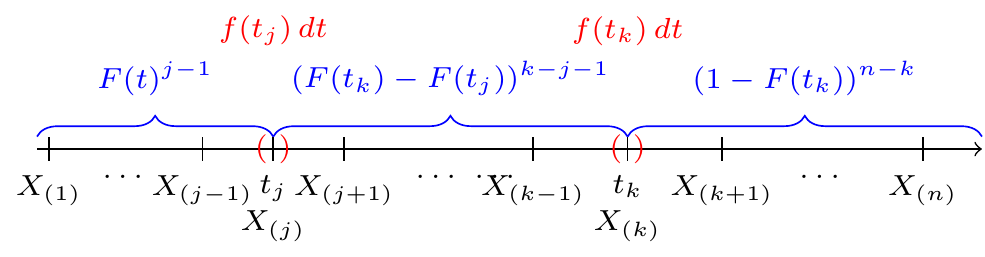
There are \[ \frac{n!}{(j-1)!1!(k-j-1)!1!(n-k)!} \] ways to arrange $X_1, \dots, X_n$ so that $j-1$ are to the left of $t_j$, $1$ is near $t_j$, $k-j-1$ are between $t_j$ and $t_k$, one is near $t_k$, and $n-k$ are to the right of $t_k$.

Then, the probability that $X_{(j)}$ and $X_{(k)}$ are near $t_j$ and $t_k$, respectively, can be approximated as \[\begin{align*} f_{X_{(j)}, X_{(k)}}&(t_j, t_k) \, \Delta t_j \, \Delta t_k \approx P\left( t_j - \frac{\Delta t_j}{2} < X_{(j)} < t_j + \frac{\Delta t_j}{2}, t_k - \frac{\Delta t_k}{2} < X_{(k)} < t_k + \frac{\Delta t_k}{2} \right) \\ &\approx \frac{n!}{(j-1)!1!(k-j-1)!1!(n-k)!} (F(t_j))^{j-1} f(t_j) (F(t_k) - F(t_j))^{k-j-1} f(t_k) (1 - F(t_k))^{n-k} \, \Delta t_j \, \Delta t_k. \end{align*}\] Dividing both sides by $\Delta t_j \Delta t_k$, we obtain Equation 41.4.

The joint PDF is useful for calculations involving more than one order statistic. For example, the interquartile range from Example 41.2 involves two order statistics, $X_{(3)}$ and $X_{(7)}$, so calculating the variance requires their joint distribution.

Example 41.3 (Variance of the interquartile range) Continuing Example 41.2, how variable is the interquartile range $X_{(7)} - X_{(3)}$?

Although we could calculate $\text{Var}\!\left[ X_{(7)} - X_{(3)} \right]$ using properties of covariance, it is easier to calculate the variance directly using the shortcut formula (Proposition 21.1): \[ \text{Var}\!\left[ X_{(7)} - X_{(3)} \right] = \text{E}\!\left[ (X_{(7)} - X_{(3)})^2 \right] - \text{E}\!\left[ X_{(7)} - X_{(3)} \right]^2. \] We already calculated the second expectation in Example 41.2. So we just need to calculate the first expectation, which requires integrating with respect to the joint PDF of $X_{(3)}$ and $X_{(7)}$. By Equation 41.4, the joint PDF is \[ f_{X_{(3)}, X_{(7)}}(u, v) = \frac{9!}{2! 3! 2!} u^2 (v - u)^3 (1 - v)^2; \qquad 0 < u < v < 1. \] Now, the first expectation is \[\begin{align} \text{E}\!\left[ (X_{(7)} - X_{(3)})^2 \right] &= \underset{0 < u < v < 1}{\iint} (v-u)^2 \cdot \frac{9!}{2! 3! 2!} u^2 (v - u)^3 (1 - v)^2\,du\,dv \\ &= \underset{0 < u < v < 1}{\iint} \frac{9!}{2! 3! 2!} u^2 (v - u)^5 (1 - v)^2\,du\,dv \\ &= \frac{5 \cdot 4}{11 \cdot 10} \underset{0 < u < v < 1}{\iint} \underbrace{\frac{11!}{2! 5! 2!} u^2 (v - u)^5 (1 - v)^2}_{\text{joint PDF of $X_{(3)}$ and $X_{(9)}$ for $n=11$}} \,du\,dv \\ &= \frac{2}{11}. \end{align}\] In the last step, we recognized that we were integrating a joint PDF of order statistics, so the integral is $1$.

Putting everything together, the variance of the interquartile range is \[ \text{Var}\!\left[ X_{(7)} - X_{(3)} \right] = \frac{2}{11} - \left(\frac{4}{10} \right)^2 = \frac{6}{275}. \]

We can derive the joint distribution of three or more order statistics in the same way. The next result states the joint distribution of all $n$ order statistics.

Proposition 41.3 (Full joint distribution of order statistics) Let $X_1, \dots, X_n$ be i.i.d. continuous random variables with PDF $f(x)$ and CDF $F(x)$. Then, the joint PDF of the order statistics is \[ f_{X_{(1)}, X_{(2)}, \dots, X_{(n)}}(t_1, t_2, \dots, t_n) = \begin{cases} n! f(t_1) f(t_2) \cdots f(t_n) & t_1 < t_2 < \dots < t_n \\ 0 & \text{otherwise} \end{cases} \tag{41.5}\]

Proof

We present another heuristic proof.

There are $n!$ ways to assign the $n$ values $X_{(1)}, \dots, X_{(n)}$ to the $n$ random variables $X_1, \dots, X_n$. Therefore, \[\begin{align*} f_{X_{(1)}, \dots, X_{(n)}} \, \Delta t_1 \cdots \Delta t_n &\approx P\left( t_1 - \frac{\Delta t_1}{2} < X_{(1)} < t_1 + \frac{\Delta t_1}{2}, \dots, t_n - \frac{\Delta t_n}{2} < X_{(n)} < t_n + \frac{\Delta t_n}{2} \right) \\ &\approx n! f(t_1) \cdots f(t_n) \, \Delta t_1 \cdots \Delta t_n, \end{align*}\] and we recover the desired PDF.

Example 41.4 (Distance between trucks) Three trucks are traveling along a 1-mile stretch of road. If each truck is equally likely to be anywhere along the stretch of road, independently of the other trucks, what is the probability that no two trucks are within $d$ miles of one another, where $0 < d < 1/3$?

Let $X_i$ denote the position of the $i$th truck. This problem is easier if we simply consider the ordered positions $X_{(i)}$, without regard to which of the three trucks it is.

By Proposition 41.3, we see that \[ f_{X_{(1)}, X_{(2)}, X_{(3)}}(t_1,t_2,t_3) = 3! \] for $0 < t_1 < t_2 < t_3 < 1$, since the PDF of $X_i$ is $1$ on $(0, 1)$.

Now, we integrate this joint PDF over the region where each truck is more than $d$ miles ahead of the previous truck. In order for this to be true,

$t_1$ must be somewhere between $0$ and $1 - 2d$ (because if the first truck were less than $2d$ miles from the end, it would be impossible for the remaining trucks to be more than $d$ miles apart from each other and the first truck),
$t_2$ must be between $t_1 + d$ ($d$ miles behind the first truck) and $1 - d$ (because if the second truck were less than $d$ miles from the end, it would be impossible to be $d$ miles ahead of the last truck), and
$t_3$ must be between $t_2 + d$ ($d$ miles behind the second truck) and $1$ (the end of the road).

Putting this into equations, we obtain \[\begin{align*} P(X_{(2)} > X_{(1)} + d, X_{(3)} > X_{(2)} + d) &= \iiint_{t_2 > t_1 + d, t_3 > t_2 + d} f_{X_{(1)}, X_{(2)}, X_{(3)}} (t_1, t_2, t_3) \, dt_1 \, dt_2 \, dt_3 \\ &= \int_0^{1-2d} \int_{t_1+d}^{1-d} \int_{t_2+d}^1 3! \, dt_3 \, dt_2 \, dt_1 \\ &= 3! \int_0^{1-2d} \int_{t_1+d}^{1-d} (1 - d - t_2) \, dt_2 \, dt_1 \\ &= 3 \int_0^{1-2d} (1-2d-t_1)^2 \, dt_1 \\ &= (1-2d)^3. \end{align*}\]

41.3 Exercises

Exercise 41.1 Let $X_1, \dots, X_n$ be i.i.d. $\text{Uniform}(0,1)$. Compute \[ P\left( X_{(k)} - X_{(k-1)} > t \right) \] for $1 \leq k \leq n+1$.

Remark. You may assume $X_{(0)} = 0$ and $X_{(n+1)} = 1$.

Exercise 41.2 (Median for an even number of observations) Let $X_1, \dots, X_n$ be i.i.d. continuous random variables. When $n$ is even, the median is defined as the average of the two middle observations: \[ \frac{X_{\left(\frac{n}{2}\right)} + X_{\left( \frac{n}{2} + 1 \right)}}{2}. \]

Repeat Example 41.1, but for $n = 10$.

Exercise 41.3 (Estimating the center of the normal distribution) Let $X_1, \dots, X_7$ be i.i.d. $\text{Normal}(\mu, \sigma)$. The MLE of $\mu$ is $\bar X$, but another estimator of $\mu$ is the sample median $X_{(4)}$.

Show that the sample median $X_{(4)}$ is also unbiased for estimating $\mu$, and compare its MSE with that of $\bar X$.

Exercise 41.4 (Estimating the center of the uniform distribution) If we observe i.i.d. random variables $X_1, \dots, X_n$ from a $\textrm{Uniform}(a= \theta - 1, b= \theta + 1)$, how do we estimate the center $\theta$? For simplicity, we will assume that $n$ is odd.

First, let $U_1, \dots, U_n$ be i.i.d. $\textrm{Uniform}(a= 0, b= 1)$. Calculate the expectation and variance of the mean $\bar U$, median $U_{\left( \frac{n+1}{2} \right)}$, and the midrange $\displaystyle \frac{U_{(1)} + U_{(n)}}{2}$.
Now, let $X_1, \dots, X_n$ be i.i.d. $\textrm{Uniform}(a= \theta - 1, b= \theta + 1)$. Calculate the MSEs of the mean $\bar X$, median $X_{\left( \frac{n+1}{2} \right)}$, and the midrange $\displaystyle \frac{X_{(1)} + X_{(n)}}{2}$ for estimating $\theta$. Which estimator is best?

Hint: Let $X_i = 2 U_i + \theta - 1$ so that you can use the results from part a.

Exercise 41.5 (Exact formula for the MSE of the median) In Example 41.1, we numerically approximated the MSE of the median of a random sample from an $\text{Exponential}(\lambda)$ distribution. Here is a way to derive the exact formula for the MSE of the median in terms of $n$.

Argue that $X_{(1)}$ and $X_{(2)} - X_{(1)}$ are independent. What are their distributions? (Hint: Use the result of Example 40.4 and the memoryless property of the exponential distribution.)
In fact, continuing this argument shows that $X_{(1)}, X_{(2)} - X_{(1)}, X_{(3)} - X_{(2)}, \dots$ are mutually independent. Use this to calculate $\text{E}\!\left[ X_{\left(\frac{n+1}{2}\right)} \right]$ and $\text{Var}\!\left[ X_{\left(\frac{n+1}{2}\right)} \right]$. (Hint: Your answer will be in the form of a summation.)
Calculate the MSE of the median for estimating the median of the exponential distribution. Your answer should be a function of $n$ and $\lambda$. Simplify as much as possible, but leave your final answer in terms of summations.