19 Expected Value
\[ \def\defeq{\overset{\text{def}}{=}} \def\E{\text{E}} \def\mean{\textcolor{red}{1.2}} \]
We define the expected value of a continuous random variable. To do this, we rely on intuition developed in Chapter 9, where expected value was defined for a discrete random variable.
19.1 Definition
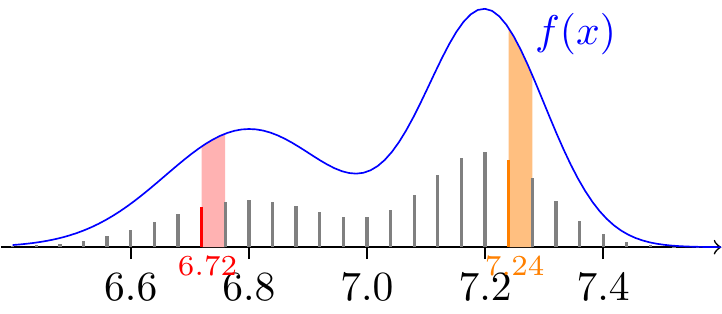
To motivate the definition of expected value for a continuous random variable, let’s consider how we might approximate it. Consider a continuous random variable \(X\) described by the PDF in Figure 19.1. If we chop up the \(x\)-axis finely enough, then we can approximate \(X\) by a discrete random variable that only takes on a discrete set of values. For example, we can represent all values in \(\textcolor{red}{[6.72, 6.76]}\) by \(\textcolor{red}{6.72}\) and all values in \(\textcolor{orange}{[7.24, 7.28]}\) by \(\textcolor{orange}{7.24}\), and we can ensure that the probability of each discrete outcome corresponds to the probability of the interval it represents.
Let \(\varepsilon\) be the spacing between values of this discrete random variable. In Figure 19.1, \(\varepsilon = 0.04\). The expected value of this discrete random variable can now be approximated as
\[ \begin{aligned} \E[X] &\approx \sum_x x \cdot P(x \leq X < x + \varepsilon) \\ &\approx \sum_x x \cdot f(x) \varepsilon. \end{aligned} \]
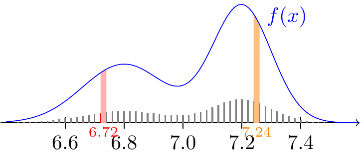
In the second line, we used Equation 18.2. We know that we can make these approximations more accurate by chopping up the \(x\)-axis finer and finer, making \(\varepsilon\) smaller and smaller. In Figure 19.2, we get a better approximation by decreasing \(\varepsilon\) to \(0.02\) because \(\textcolor{red}{6.72}\) now only represents the smaller interval \(\textcolor{red}{[6.72, 6.74]}\) and \(\textcolor{orange}{7.24}\) only represents \(\textcolor{orange}{[7.24, 7.26]}\).
In the limit as \(\varepsilon \to 0\), this Riemann sum becomes an integral:
\[ \sum_x x \cdot f(x) \varepsilon \to \int_{-\infty}^\infty x f(x)\,dx. \]
This is the motivation behind the definition of the expected value of a continuous random variable.
Just as the expected value of a discrete random variable was where the PMF would balance, the expected value of a continuous random variable is where the PDF would balance on a scale. – is center of mass.
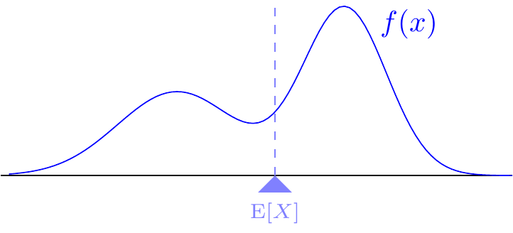
This center of mass interpretation can be used to bypass Equation 19.1 in some situations, as illustrated in the next example.
Example 19.1 (Expected Long Jump Distance) In Example 18.3, we examined a uniform model for \(X\), the distance of one of Joyner-Kersee’s long jumps. The PDF of \(X\) is \[ f(x) = \begin{cases} \frac{1}{1.2} & 6.3 < x < 7.5 \\ 0 & \text{otherwise} \end{cases}, \] which looks like this:
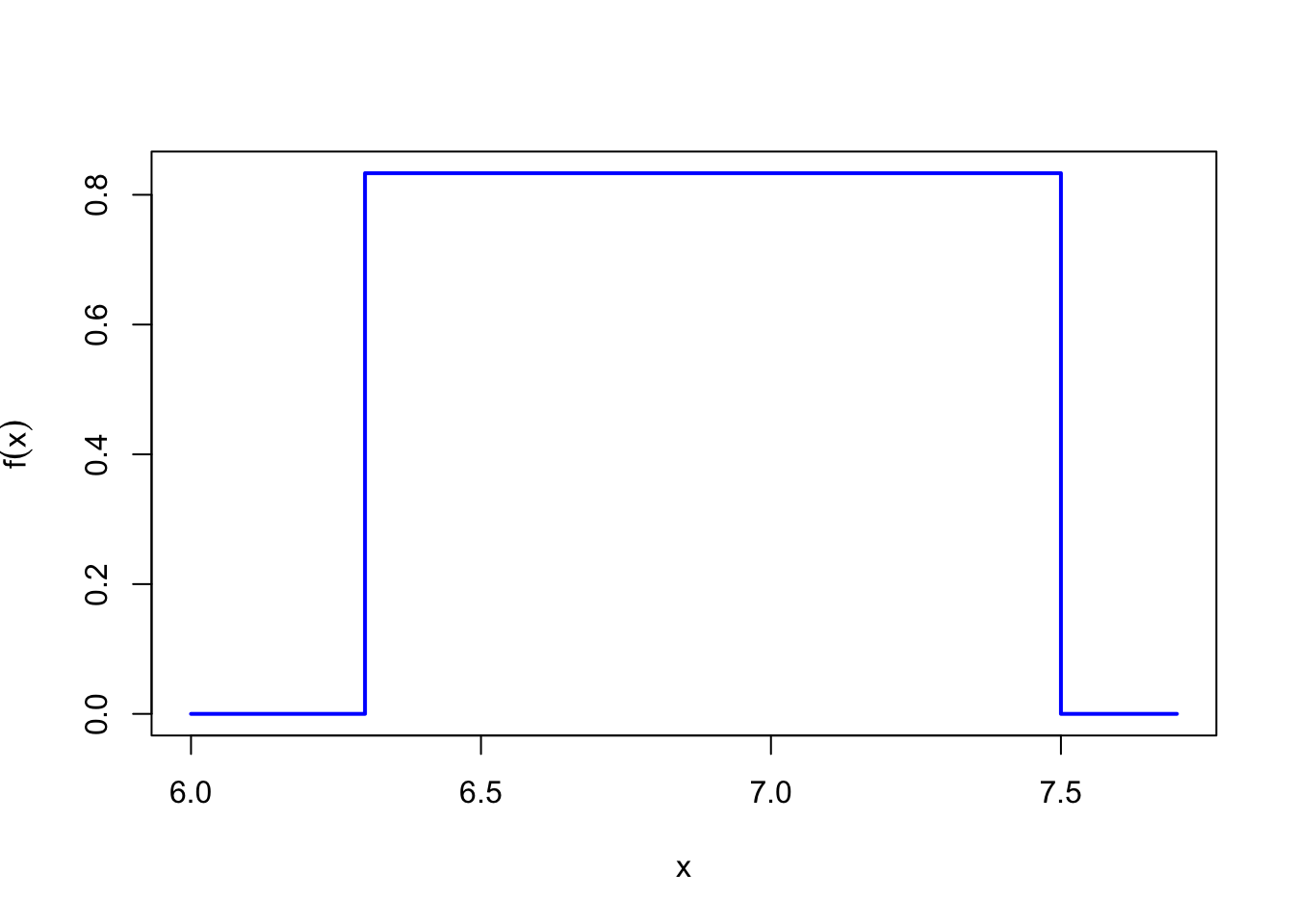
Under this model, what is \(\E[X]\), the expected distance of her long jump?
Because of symmetry, this PDF could only balance at the midpoint of the support, so the center of mass (and expected value) must be \[ \E[X] = \frac{6.3 + 7.5}{2} = 6.9\ \text{meters}. \]
We can check this answer using Equation 19.1: \[ \begin{aligned} \E[X] &= \int_{6.3}^{7.5} x \cdot \frac{1}{1.2}\,dx \\ &= \frac{1}{1.2} \cdot \frac{x^2}{2} \Big|_{6.3}^{7.5} \\ &= \frac{1}{1.2} \left( \frac{7.5^2}{2} - \frac{6.3^2}{2} \right) \\ &= 6.9, \end{aligned} \] but the center of mass interpretation allowed us to bypass the calculus.
However, in most situations, the center of mass will not be obvious, and we will need to use Equation 19.1 to determine the expected value.
19.2 Case Study: Radioactive Particles
Let’s apply Definition 19.1 to the Geiger counter example from Section 18.3.
Calculating the integral in Example 19.2 was rather messy. The next result makes expected values like this one easier to calculate. It is the direct analog of Proposition 9.3.
Let’s apply Proposition 19.1 to determine the expected time of the first arrival.
Another way to summarize a random variable is the median.
In the next example, we see that the median is not the same as the expected value (which is also called the mean).
19.3 When the Expected Value Does Not Exist
The expected value is not well-defined for all random variables. In Section 9.4, we saw examples of random variables whose expected value was infinite; the next example provides an example of a random variable whose expected value is not well-defined at all.
Example 19.5 (A distribution without an expected value) A random variable \(X\) is said to follow a Cauchy distribution if its PDF is \[ f_X(x) = \frac{1}{\pi} \cdot \frac{1}{1 + x^2}; \qquad -\infty < x < \infty. \] This PDF is graphed below. It is easy to check that \(f_X(x)\) is a valid PDF that integrates to one.
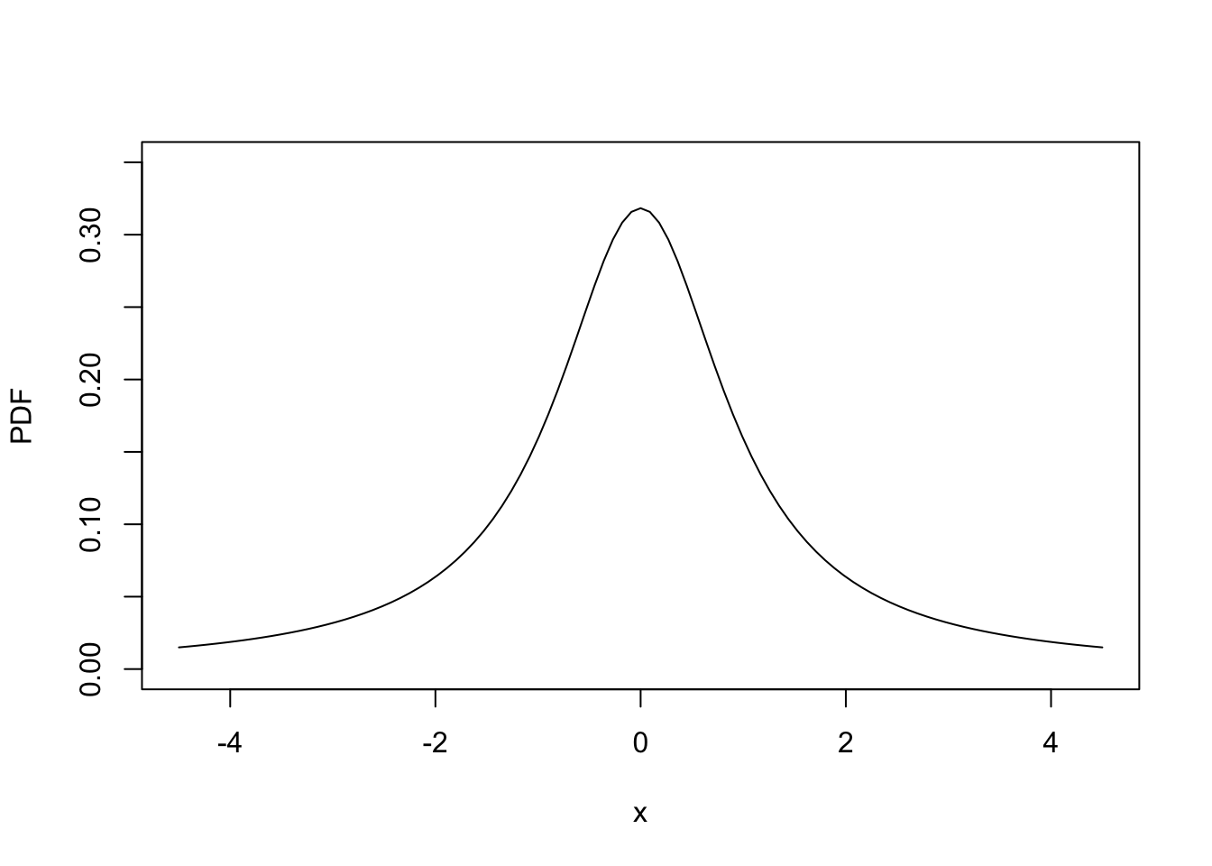
At first glance, it seems that the expected value of \(X\) should be \(0\), by symmetry. However, the expected value does not exist because if it did, then it would have to equal \[ \begin{align} \E[X] &= \int_{-\infty}^\infty x \cdot \frac{1}{\pi} \cdot \frac{1}{1 + x^2}\,dx \\ &= \lim_{a\to-\infty} \int_{a^2}^0 \frac{1}{\pi} \cdot \frac{x}{1 + x^2}\,dx + \lim_{b\to\infty} \int_0^{b^2} \frac{1}{\pi} \cdot \frac{x}{1 + x^2}\,dx \\ &= \lim_{a\to-\infty} \int_{a^2}^0 \frac{1}{2\pi} \cdot \frac{1}{1 + u}\,du + \lim_{b\to\infty} \int_0^{b^2} \frac{1}{2\pi} \cdot \frac{1}{1 + u}\,du, \\ \end{align} \] where we used the substitution \(u = x^2\).
The first limit diverges to \(-\infty\), while the second limit diverges to \(\infty\). Therefore, the expected value is undefined; it cannot converge to a finite number, nor can it diverge to \(\pm\infty\).
19.4 Exercises
Exercise 19.1 (Expected temperature in Iqaluit) In Example 18.5, we saw that the temperature in Iqaluit (in Celsius) could be modeled as a continuous random variable \(C\) with PDF \[ f_C(x) = \frac{1}{k} e^{-x^2/18}; -\infty < x < \infty. \]
Determine the expected temperature in Iqaluit, \(\E[C]\), in two ways:
- using symmetry
- using Definition 19.1.
Exercise 19.2 (When does the mean equal the median?) In Example 19.4, we saw that the mean is not the same as the median in general. However, here is one situation where the mean and median are equal.
Suppose the PDF \(f_X(x)\) of a continuous random variable \(X\) is symmetric. That is, suppose there exists \(m\) such that for all \(t > 0\), \[ f_X(m + t) = f_X(m - t). \tag{19.3}\]
Show that if the mean \(\E[X]\) exists, it must equal the median.
Exercise 19.3 (The Pareto distribution and incomes) In economics, the Pareto distribution is used to model incomes and study income inequality. (Jones 2015) The Pareto distribution has PDF \[ f(y) = \begin{cases} \frac{\alpha \ell^\alpha}{y^{\alpha+1}} & y \geq \ell \\ 0 & \text{otherwise} \end{cases}, \tag{19.4}\] where \(\alpha > 0\) is an “inequality” parameter and \(\ell\) is the minimum income.
- Let \(Y\) be the income of a random selected worker. Calculate \(\E[Y]\), the average income of a worker. For what values of \(\alpha\) is this finite?
- What percentage of total income is earned by the top 1% of workers? (Hint: You may assume that the number of workers is \(N\); however, all \(N\)s and \(\ell\)s should cancel out in the end so that you end up with an answer that only depends on \(\alpha\).)
Note: In the United States, \(\alpha\) is approximately \(5/3\).
Exercise 19.4 (Lorenz curve and Gini coefficient) This exercise is a continuation of Exercise 19.3. Suppose that incomes are distributed according to a Pareto distribution (Equation 19.4), where \(\alpha\) is chosen so that \(\E[Y] < \infty\).
- The Lorenz curve \(L(p)\) is defined to be the fraction of total income earned by the lowest proportion \(p\) of workers. Calculate \(L(p)\) in terms of \(\alpha\). (Hint: Although in principle \(L(p)\) could depend on the minimum income \(\ell\), it does not.) Graph the curve for different values of \(\alpha\). What do the limits \(\alpha = 1\) and \(\alpha = \infty\) correspond to?
- Note that the Lorenz curve \(L(p) = p\) corresponds to perfect income equality. Therefore, income inequality in a population can be measured by the area between this line and the Lorenz curve. The Gini coefficient is defined as the area between these two curves, normalized so that the maximum is \(1\): \[ G = \frac{\text{area between Lorenz curve and line of perfect income equality}}{\text{total area under line of perfect income inequality}}. \tag{19.5}\] Calculate the Gini coefficient as a function of \(\alpha\). In the United States, \(\alpha\) is approximately \(5/3\). What is the Gini coefficient for the U.S.?