2 Techniques for Counting

To apply the classical definition of probability, we need to count the number of outcomes in the sample space and in the event of interest. For the examples in Chapter 1, we did so by explicitly listing out the relevant outcomes (e.g., see Figure 1.9). But in this chapter, we will encounter events and sample spaces so large that listing out every outcome is impractical. To tackle these more difficult problems, we will need tools from combinatorics, the branch of mathematics concerned with counting.

Like probability, combinatorics is a tricky subject that can be daunting and counterintuitive at first. But once you learn a few basic principles, you will be able to tackle a wide variety of probability problems involving counting.

2.1 The Fundamental Principle of Counting

We open with a simple everyday example that illustrates the core idea behind counting.

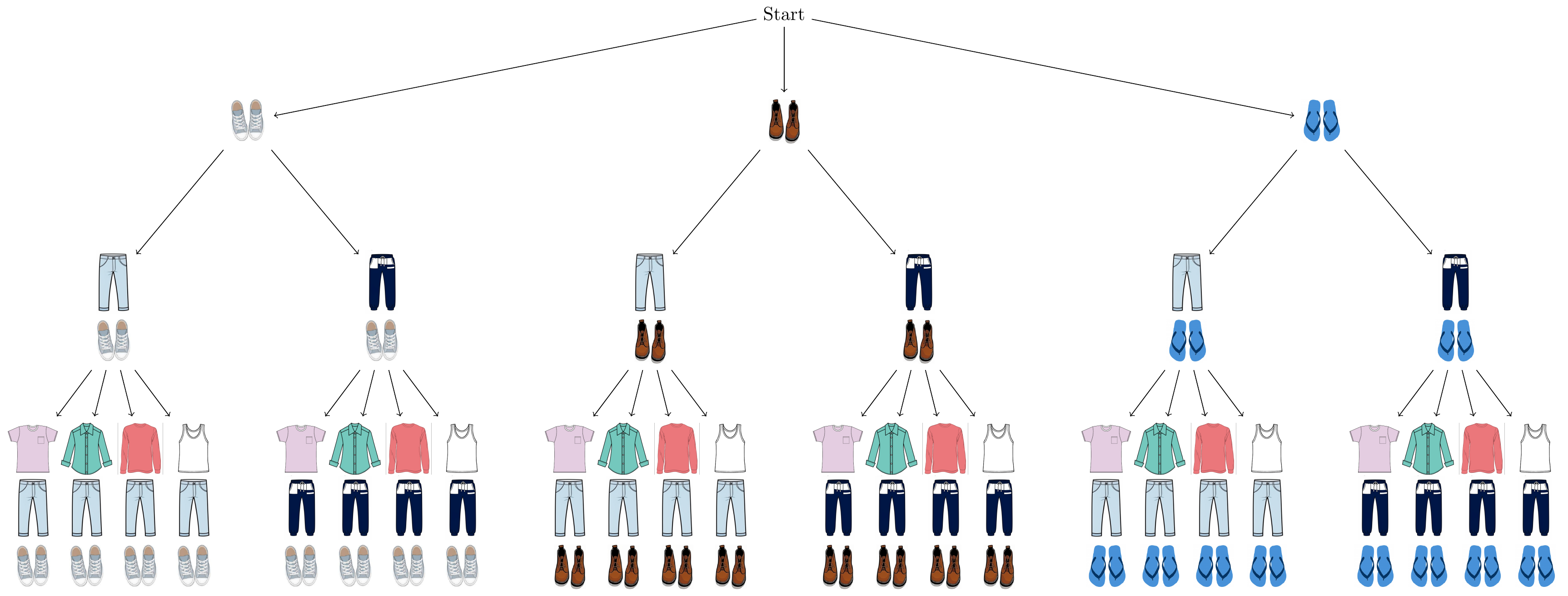
Example 2.1 (Random outfits) Suppose our outfit for the day is composed of three clothing items: shoes, pants, and a shirt. We have three pairs of shoes, two pairs of pants, and four different shirts. Two of our shirts are long-sleeved, and the other two are not. If we randomly toss together an outfit (i.e., each possible outfit is equally likely), what is the probability that we wear a long-sleeved shirt?

To compute the probability of the event \(A\) that we wear a long-sleeved shirt, we first need to

count the number of outcomes in the sample space \(\Omega\),
count the number of outcomes in the event \(A\).

Then we can easily apply the classical definition of probability (Definition 1.3) to compute \(P(A)\).

How many possible outcomes are there?

The sample space \(\Omega\) is composed of all the possible outfits we can make. How many such outfits are there? Each of the \(3\) pairs of shoes can be matched with \(2\) possible pairs of pants, making \(2 \times 3 = 6\) shoe and pant combos. For each of these \(6\) shoe and pant combos, there are \(4\) different shirts we can wear, making for a total of \(2 \times 3 \times 4 = 6 \times 4 = 24\) unique outfits. Figure 2.1 both illustrates this line of reasoning and enumerates all the outfits in the sample space.

Figure 2.1: Visual enumeration of all the possible outfits.

How many outcomes are in \(A\)?

We can apply the same reasoning to count the number of outfits with long-sleeved shirts. There are \(2\) long-sleeved shirts that can be paired with \(2 \times 3 = 6\) pant and shoe combos, making for a total of \(2 \times 2 \times 3 = 12\) outfits with long-sleeved shirts. Figure 2.1 affirms our argument.

Applying the classical definition of probability

Combining these facts, we can apply the classical definition of probability (Definition 1.3) to compute \(P(A)\):

\[ P(A) = \frac{|A|}{|\Omega|} = \frac{12}{24} = .5. \]

Recognizing symmetry

Since \(2\) of the \(4\) shirts are long-sleeved, it perhaps came as no surprise that the probability wearing a long-sleeved shirt was equal to \(P(A) = 2/4 = .5\).

This is an example of the general principle of symmetry. There is no reason that one shirt should be more likely than any other, since every outfit is equally likely. Therefore, the probability of wearing a long-sleeved shirt must be \(2 / 4\), the number of long-sleeved shirts divided by the total number of shirts.

Symmetry is a powerful tool that allows us to circumvent lengthy arguments. Correspondingly, we will appeal to it throughout this book.

In Example 2.1, we used the following principle.

Theorem 2.1 (The fundamental principle of counting) Suppose \(n\) consecutive actions are performed and, regardless of the previously taken actions, there are \(k_i\) distinct ways to perform the \(i\)th action. Then, there are \[ \prod_{i=1}^{n} k_i = k_1\times \dots \times k_n \tag{2.1}\] unique ways to perform the \(n\) actions.

In Example 2.1, we made outfits by performing three actions: choosing a pair of shoes, choosing a pair of pants, and choosing a shirt. Each way of performing the actions results in a unique outfit, and each possible outfit results from a unique way of performing the actions. Consequently, the number of possible outfits is equal to the number of unique ways to perform these actions. Since there are \(3\) ways to perform the first action, then always \(2\) ways to perform the second, and then always \(4\) ways to perform the third, Theorem 2.1 implies that there are \(2 \times 3 \times 4 = 24\) unique ways of performing the actions, and hence \(24\) possible outfits. Check for yourself that, even if the shoes, pants, and shirt had been picked in a different order (e.g., first pick the pants, then shirt, then shoes), we would have obtained the same answer.

2.2 Four Ways of Counting

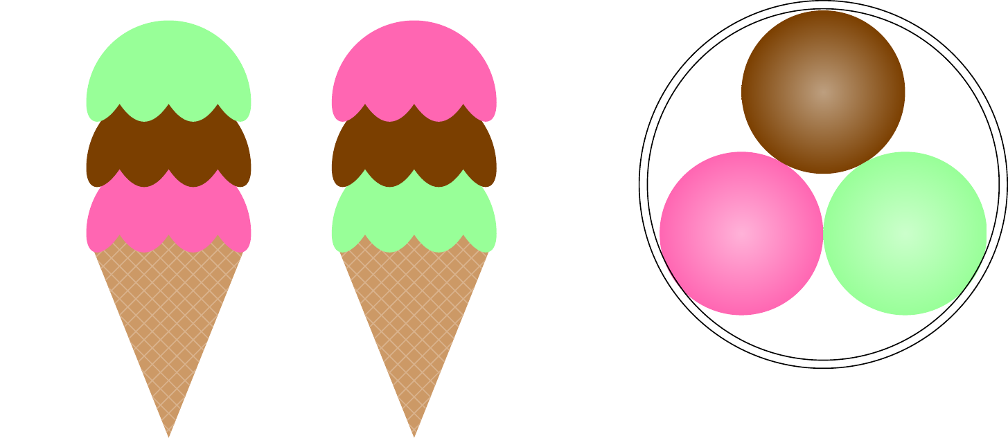
Many counting problems in probability take the form of: “How many ways are there to pick \(k\) items from \(n\) (unique) items?” For example, consider a local ice cream shop that offers \(n=5\) flavors. They allow customers to pick \(k=3\) scoops. How many distinct ice cream “experiences” are there?

Figure 2.2: Ice cream flavors offered at the local ice cream shop.

Unfortunately, this question is ambiguous as stated. First, it depends on whether or not order matters—that is, whether the ice cream is in a cone or a cup. In a cone, the experience depends on the order of the scoops; eating chocolate after mint is a different experience from eating mint after chocolate, and the cone is consumed with whichever flavor is on the bottom. In a cup, the order of the flavors does not affect the experience, since all scoops are equally accessible.

Figure 2.3: Order matters in a cone, but not in a cup.

There is also the matter of whether the items are selected with or without replacement—that is, whether there can be multiple scoops of the same flavor. There will be more possible ice cream experiences if a flavor can be picked multiple times.

2.2.1 Order Matters: Ice Cream in a Cone

When scoops of ice cream are in a cone, the order of the scoops matters. \((\text{mint}, \text{chocolate}, \text{strawberry})\) is a distinct experience from \((\text{strawberry}, \text{chocolate}, \text{mint})\). How do we count the total number of distinct experiences?

2.2.1.1 Picking with Replacement

If we allow the possibility of picking the same flavor multiple times, then there are \(5\) options for the first scoop, \(5\) options again for the second scoop, and \(5\) options still for the last scoop. By the Fundamental Principle of Counting (Theorem 2.1), the number of distinct experiences when selecting with replacement is \[ 5 \times 5 \times 5 = 5^3 = 125. \]

This is a special case of a more general rule.

Proposition 2.1 (Counting ordered selections with replacement) If there are \(n\) unique items, then the number of ordered ways to select \(k\) items with replacement is \[n^k.\]

Proposition 2.1 is especially handy in probability problems where the same action is repeated over and over, such as rolling a die multiple times. In the next example, we use Proposition 2.1 to correctly solve Example 1.1, a problem that Cardano himself solved incorrectly. Cardano had reasoned that it would take \(n=3\) rolls of a fair die to have an even chance of rolling a six.

Solution 2.1 (Solving Cardano’s problem). We will rephrase Cardano’s problem. What is the probability of not rolling any sixes in \(n\) rolls?

How many possible outcomes are there?

The possible outcomes of \(n\) rolls of a die correspond to the different ways of selecting \(n\) items from \(\{ 1, 2, 3, 4, 5, 6\}\). The selection is with replacement because it is possible to roll the same number twice. Proposition 2.1 says that there are \(6^n\) ways to make this selection, and therefore \(6^n\) total outcomes.

How many outcomes have no sixes?

The outcomes with no sixes correspond to the different ways of selecting \(n\) items from \(\{1, 2, 3, 4, 5\}\) with replacement. Proposition 2.1 says that there are \(5^n\) such outcomes.

Applying the classical definition of probability

Applying the classical definition of probability (Definition 1.3), we find that \[ P(\text{no sixes}) = \frac{5^n}{6^n}. \]

The code below graphs this probability for different values of \(n\) and thereby answers Cardano’s question.

The plot shows that \(n=4\) rolls is where the chance of rolling no sixes crosses below 50%, so this is also where the chance of rolling one or more sixes is first above 50%.

2.2.1.2 Picking without Replacement

What if we do not allow the possibility of picking the same flavor multiple times? We can count the number of ways to pick three distinct flavors as follows: there are \(5\) options for the first scoop, \(4\) options for the second scoop (because it must be one of the other four flavors), and only \(3\) options for the last scoop. By the Fundamental Principle of Counting (Theorem 2.1), the number of distinct experiences when selecting without replacement is \[ 5 \times 4 \times 3 = 60. \]

We can write this expression more compactly with the help of factorials. Recall that \(n!\) (pronounced “\(n\) factorial”) is defined to be the product of the integers from \(n\) down to \(1\): \[ n! = n \times (n-1) \times \dots \times 1. \] (By convention, \(0!\) is defined to be \(1\).) Using factorials, we can write \[ 5 \times 4 \times 3 = \frac{5!}{2!}. \]

The same reasoning extends to any ordered selection of \(k\) items from a collection of \(n\) unique items.

Proposition 2.2 (Counting ordered selections without replacement) If there are \(n\) unique items, then the number of ordered ways to select \(k\) items without replacement is \[\frac{n!}{(n-k)!}.\]

Proposition 2.2 can be used to count the number of ways of arranging \(n\) items. A particular arrangement or ordering of items is called a permutation of the items.

Corollary 2.1 (Number of permutations) There are \(n!\) permutation of \(n\) distinct objects.

Proof

Ordering \(n\) objects corresponds exactly to selecting all \(n\) items (from the set of \(n\) items) without replacement, where order matters. Proposition 2.2 says that there are \(\frac{n!}{(n-n)!} = \frac{n!}{0!} = n!\) ways of doing so.

Corollary 2.1 can be applied to Secret Santa (Example 1.7).

Example 2.2 (A Secret Santa disaster) Recall the Secret Santa gift exchange from Example 1.7. What is the probability of the worst-case event, where everyone draws their own name?

How many possible outcomes are there?

In Example 1.7, we represented each outcome as an ordering of the four numbers \(\{ 1, 2, 3, 4 \}\). For example, the outcome \(2134\) means that friends 3 and 4 drew their own name, but friend 1 drew friend’s 2 name and friend 2 drew friend 1’s name.

By Corollary 2.1, there are \(4! = 4 \cdot 3 \cdot 2 \cdot 1 = 24\) ways to order these four numbers.

In how many outcomes does every friend draw their own name?

There is only one outcome, \(1234\), where every friend draws their own name.

Applying the classical definition of probability

Putting these facts together, we can apply the classical definition of probability (Definition 1.3) to see that \[ P(\text{everyone draws their own name}) = \frac{1}{4!} = \frac{1}{24}. \]

The last example is a classic probability brainteaser with a surprising answer. It makes use of both Proposition 2.1 and Proposition 2.2.

Example 2.3 (Birthday Problem) In a room of \(k\) randomly selected people, what is the probability that at least two people share a birthday? Alternatively, what is the probability that no one shares a birthday?

First, we’ll make two simplifying assumptions:

We only select people born during the standard \(365\) day calendar year (with apologies to people born on leap day!).
All configurations of the \(n\) people’s birthdays are equally likely.

How many possible outcomes are there?

Imagine ordering the people in the room. The number of different birthday configurations is the number of ordered ways to select \(k\) days from the \(365\) days of the year, with replacement because it is possible for two people to have the same birthday. The first selection is the birthday of the first person in the ordering, the second selection is the birthday of the second person, so on and so forth. Proposition 2.1 says that there are \(365^k\) ways to perform this selection, and therefore \(365^k\) total outcomes.

How many outcomes are there where no one shares a birthday?

The number of configurations where nobody shares the same birthday is the same as the number of ordered ways we can select \(k\) days from the \(365\) days of the year, without replacement to guarantee that the birthdays are all different. Proposition 2.2 says that there are \(\frac{365!}{(365 - k)!}\) ways to do so.

Applying the classical definition of probability

Applying the classical definition of probability (Definition 1.3), we find that the probability that no one shares a birthday is \[ P(\text{no one shares a birthday}) = \frac{\frac{365!}{(365 - k)!}}{365^k}. \]

This is difficult to evaluate by hand, but easy on a computer. For a room of \(k=40\) people, this probability is:

This probability is only around 10%. In other words, even in a room with just 40 people, there is already more than a 90% chance that two people will share a birthday.

In fact, it only takes \(k=23\) people for there to be a more than \(50\%\) chance of a shared birthday! Verify this for yourself by editing code above.

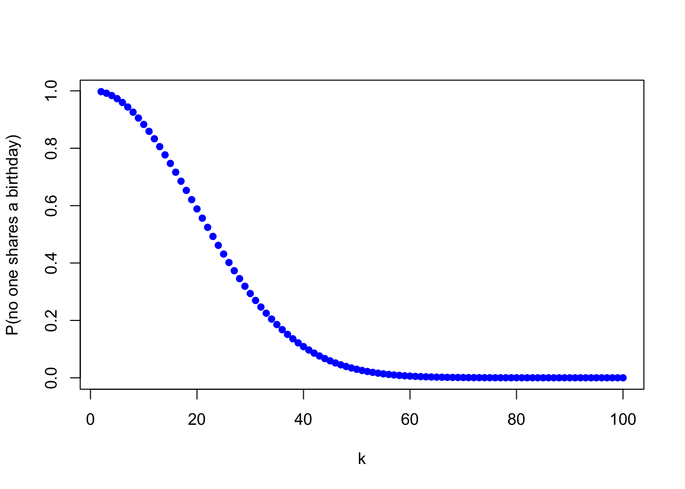
To better understand how this probability varies as a function of the number of people in the room, the graph below shows \(P(\text{no one shares a birthday})\) for \(k\) ranging from \(2\) to \(100\).

2.2.2 Order Doesn’t Matter: Ice Cream in a Cup

When ice cream is in a cup, the order of the scoops does not matter. How many distinct ice cream experiences are there if the scoops are in a cup?

2.2.2.1 Picking without Replacement

First, we consider the case where the flavors are chosen without replacement; that is, when the scoops must be of different flavors. To count the number of distinct experiences, we will first count the number of ordered experiences and then adjust for double counting.

In Section 2.2.1, we showed that there were \(\frac{5!}{2!} = 60\) distinct experiences with a cone, when the scoops were required to be of different flavors. We list these \(60\) experiences in Figure 2.4. We arrange this list so that different reorderings of the same three flavors are in the same row.

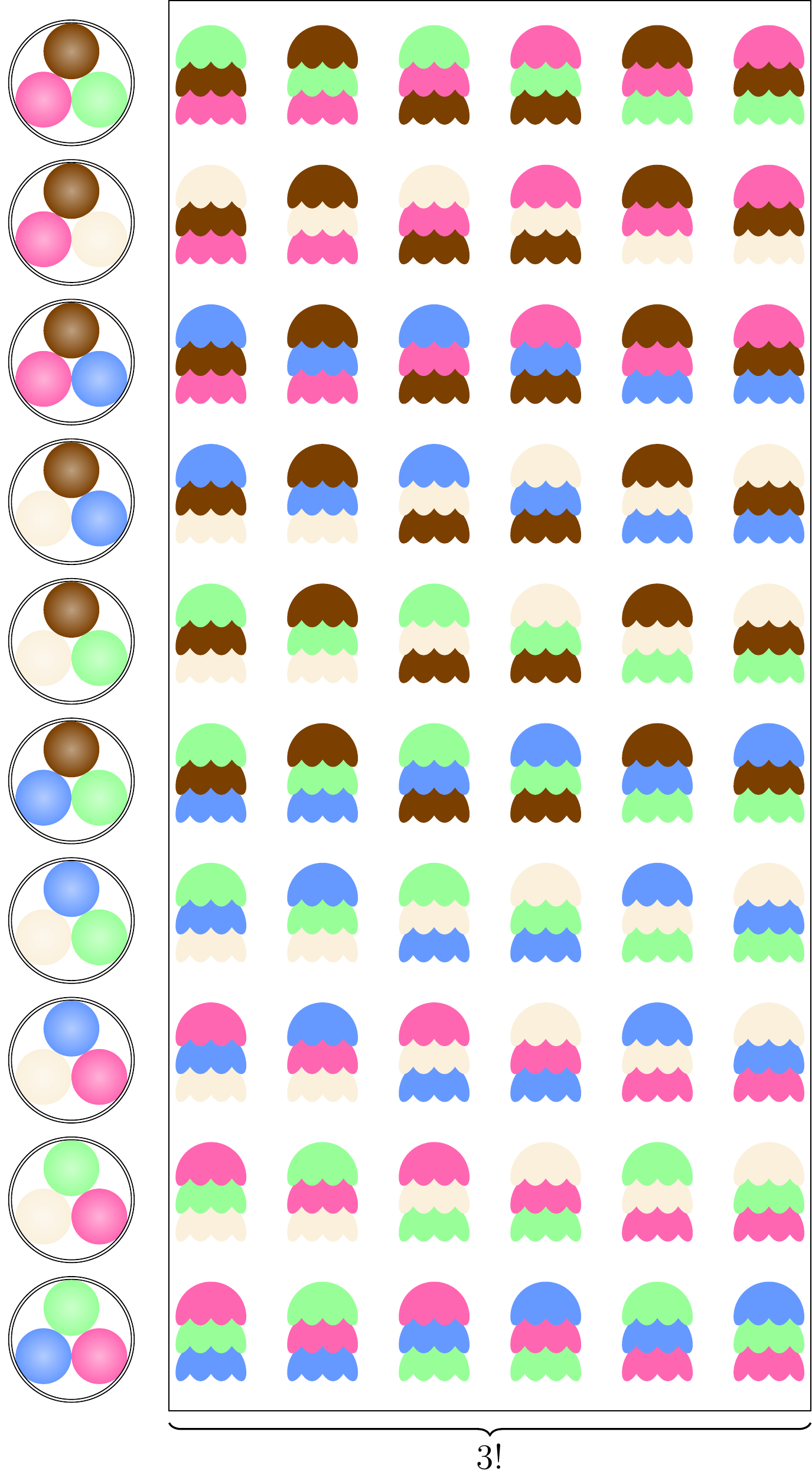
Figure 2.4: The \(60\) distinct experiences in a cone and \(10\) distinct experiences in a cup.

In Figure 2.4, we know that the rectangle contains \(\frac{5!}{2!} = 60\) distinct ordered experiences, by Proposition 2.2. However, we want to count the number of distinct unordered experiences, which corresponds to the number of rows in the rectangle. Since each row contains \(3! = 6\) ordered experiences (because there are \(3!\) ways to order the same three flavors), we can simply divide \(\frac{5!}{2!}\) by \(3!\) to obtain the number of rows: \[ \frac{5!}{3! 2!} = 10. \]

Generalizing this argument to any \(n\) and \(k\), we know that there are \(\frac{n!}{(n-k)!}\) ordered ways to select \(k\) items from \(n\) without replacement, but this double-counts each set of items \(k!\) times. Therefore, we divide by \(k!\) to obtain the number of unordered ways to select \(k\) items from \(n\).

Proposition 2.3 (Counting unordered selections without replacement) If there are \(n\) unique items, then the number of unordered ways to select \(k\) items without replacement is \[ \frac{n!}{k! (n-k)!}. \]

This expression appears so frequently in counting problems that it has its own a shorthand: \[ {n \choose k} \overset{\text{def}}{=}\frac{n!}{k! (n-k)!}, \tag{2.2}\] read as “\(n\) choose \(k\).” Equation 2.2 is called a binomial coefficient because it appears in the binomial theorem (see Exercise 2.21); it is sometimes also called a combination.

One situation where it is natural to consider unordered outcomes is in the card game poker. In poker, each player is dealt a hand of five cards from a shuffled deck of playing cards, such as the one shown in Example 1.5. The player with the “best” hand wins. (In poker, the hands are ranked based on their probability; rarer hands are considered better. For a list of poker hands, please refer to this Wikipedia article.)

In the next example, we calculate the probability of a full house, one of the best hands in poker. Notice that the order of the five cards in the hand does not matter, which is why Proposition 2.3 applies.

Example 2.4 (Probability of a full house) What is the probability of being dealt a full house in poker?

How many different five-card hands are there?

The number of five-card hands is the number of unordered ways to choose \(k=5\) cards from the \(n=52\) card deck without replacement. By Proposition 2.3, there are \(52 \choose 5\) ways to do so.

How full houses are there?

Counting the number of full houses is a bit more involved. A full house is any hand composed of

three cards of one rank (a set), and
two cards of another rank (a pair).

Each way of taking the following four consecutive actions corresponds to a unique full house, and vice-versa:

From the \(13\) different ranks, choose the rank of the set. There are \({13 \choose 1} = 13\) ways to do this.
From the \(4\) different suits, choose \(3\) for the cards in our set. There are \({4 \choose 3} = 4\) ways to do this.
From the \(12\) remaining ranks that have not been selected yet, choose the rank of the pair. There are \({12 \choose 1} = 12\) ways to do this.
From the \(4\) possible suits, choose \(2\) suits for the cards in our pair. There are \({4 \choose 2} = 6\) ways to do this.

By Theorem 2.1, the number of full houses is therefore \[{13 \choose 1} \cdot {4 \choose 3} \cdot {12 \choose 1} \cdot {4 \choose 2} = 13 \cdot 4 \cdot 12 \cdot 6 = 3744. \]

Applying the classical definition of probability

Applying the classical definition of probability (Definition 1.3), we find that the probability of being dealt a full house is \[P(\text{full house}) = \frac{3744}{{52}\choose{5}} \approx 0.0014. \] The chance of getting a full house is only about \(0.14\%\), which is why it is considered one of the best hands in poker.

We can also use Proposition 2.3 to address a common misconception about the frequentist interpretation of probability introduced in Chapter 1. To say that a coin has a \(.5\) probability of landing heads means that if we were to toss the coin \(n\) times, then the proportion of heads will approach \(.5\) as \(n\) grows. It does not mean that the number of heads will approach \(.5 n\), as the next example shows.

Example 2.5 (Exactly half of the tosses are heads) Suppose a fair coin is tossed \(n = 2k\) times. What is the probability that exactly half (i.e., \(k\)) of these tosses are heads?

How many possible outcomes are there?

The number of outcomes is the number of ordered ways to pick \(n = 2k\) items from \(\{\)H\(,\) T\(\}\). The selection is with replacement (of course, since there are only two items to select). By Proposition 2.1, there are \(2^{2k}\) ways.

In how many outcomes are exactly half the flips heads?

We want to count the number of outcomes with exactly \(k\) heads. For example, if \(n = 2k = 8\), then examples of outcomes include

HTHTHTHT
HHHHTTTT
HTTHTTHH

(and so on…)

To count the number of such outcomes, we consider choosing the positions of the \(k = 4\) heads from the \(n = 8\) tosses. That is, we are selecting \(k = 4\) items from the set \(\{ 1, 2, 3, 4, 5, 6, 7, 8 \}\) without replacement (since it is impossible to have two heads on one toss). Outcome 1 would correspond to selecting \(\{ 1, 3, 5, 7 \}\), while outcome 2 would correspond to selecting \(\{ 1, 2, 3, 4 \}\).

By Proposition 2.3, there are \({{2k} \choose {k}}\) ways to choose the positions of the \(k\) heads from among the \(n = 2k\) tosses.

Applying the classical definition of probability

Applying the classical definition of probability (Definition 1.3), we find that \[P(\text{exactly } k \text{ heads}) = \frac{2k \choose k}{2^{2k}}. \tag{2.3}\]

Discussion

What happens as the number of tosses \(n = 2k\) grows? The code below calculates the probability in Equation 2.3 for up to \(n = 100\) tosses.

In fact, not only is the probability decreasing as the coin is tossed more, but it in fact decreases to zero!

To obtain some intuition for why this probability is so small, we graph the probability of obtaining exactly \(k\) heads in \(n = 100\) tosses for \(k = 0, 1, \dots, n\) below. As we ask you to show in Exercise 2.10, this probability is \[P(\text{exactly } k \text{ heads}) = \frac{n \choose k}{2^{n}}.\]

When a coin is tossed \(n=100\) times, \(k=50\) heads is indeed more probable than any other value, but there are so many values near \(50\) that the probability of exactly \(50\) is low. This effect becomes more pronounced as \(n\) increases. Try increasing \(n\) in the code above to see what happens.

2.2.2.2 Picking with Replacement

What if the flavors had been selected with replacement? That is, what if we allow multiple scoops of the same flavor? Clearly, there would be more ice cream cup experiences than the \(\binom{5}{3} = 10\) experiences above. We also have to count the possibility of two scoops of strawberry and one scoop of chocolate, or even the possibility of three scoops of mint, as illustrated in Figure 2.5. These scoops are in a cup, so order still does not matter.

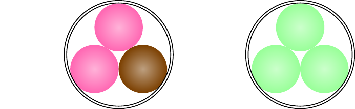
Figure 2.5: Additional ice cream cup experiences when flavors are selected with replacement.

Counting the number of distinct experiences requires a touch of ingenuity. First, when order does not matter, each experience can be summarized by reporting the number of scoops of each flavor. We can create \(5\) bins, one for each flavor, using \(4\) “bars,” as shown below: \[ \phantom{*}\underbrace{}_{\text{vanilla}} \big| \phantom{*}\underbrace{}_{\text{chocolate}} \big| \phantom{*}\underbrace{}_{\text{strawberry}} \big| \phantom{*}\underbrace{}_{\text{blueberry}} \big| \phantom{*}\underbrace{}_{\text{mint}}. \] Next, we will represent each scoop by a “star.” For a cup with \(3\) scoops, there will be \(3\) stars. For example, the two cups in Figure 2.5 would be represented by the pictures \[ \begin{align} \big|\ *\ \big| * *\ \big|\ \big| & & \text{and} & & \big|\ \big| \ \big|\ \big|\ * * *. \end{align} \] Now, the question is how many possible “stars and bars” pictures can we draw, consisting of \(3\) stars and \(4\) bars? Since there are \(7\) total objects, and we need to choose the positions of the \(3\) stars, there are \[ \binom{7}{3} = \frac{7!}{3! 4!} = 35 \] distinct cup experiences if we can have multiple scoops of the same flavor. Equivalently, we could have chosen the positions of the \(4\) bars and obtained the same answer: \[ \binom{7}{4} = \frac{7!}{4! 3!} = 35. \] The fact that these two binomial coefficients have the same value is no accident, as you will show in Exercise 2.18.

We can use the same “stars and bars” argument for any \(n\) and \(k\). If there are \(n\) flavors, then there will be \(n-1\) bars and \(k+n-1\) total objects to arrange.

Proposition 2.4 (Counting unordered selections with replacement) If there are \(n\) unique items, then the number of unordered ways to select \(k\) items with replacement is \[ \binom{k+n-1}{k} = \binom{k+n-1}{n-1}. \]

However, Proposition 2.4 is less useful than Proposition 2.3 in probability theory. This is because unordered outcomes are usually not equally likely when items are selected with replacement. Leibniz’s mistake in Example 1.2 essentially arose from trying to use Proposition 2.4 to calculate probabilities.

Leibniz’s error reconsidered

In Example 1.2, we considered the following problem: if two fair dice are thrown, is an eleven or a twelve more likely?

Leibniz erred by counting the unordered outcomes of two dice. That is, he counted the ways to select \(2\) numbers from \(\{ 1, 2, 3, 4, 5, 6 \}\), ignoring the order of the numbers. This is why he concluded that there was only one way to roll an eleven; if we ignore order, then the only way to roll an eleven is to roll a \(5\) and a \(6\).

By Proposition 2.4, there are \({7 \choose 2} = \frac{7!}{2! 5!} = 21\) distinct outcomes of two dice, ignoring order. Verify this for yourself in Figure 1.9. By Leibniz’s reasoning, the probability of an eleven and the probability of a twelve would both be equal to \(\frac{1}{21}\).

This reasoning is wrong because the unordered outcomes of two dice are not equally likely. As we have seen, rolling any two distinct numbers (such as \(5\) and \(6\)) is twice as likely as rolling any particular double (such as \(6\) and \(6\)). This is because there are \(2\) ways to order two distinct numbers but only \(1\) way to order two of the same number.

In order to correctly calculate probabilities, we must count ordered outcomes, as we did in Solution 1.1.

2.2.3 Summary

How many ways are there to to pick \(k\) items from \(n\) (unique) items? The answer to this question depends on

whether order matters or not, and
whether items are selected with or without replacement.

In this section, we determined the answer to all four cases, and the formulas are summarized in Table 2.1.

Table 2.1: Number of ways to select \(k\) items from a collection of \(n\) unique items

	Order Matters	Order Doesn’t Matter
Without Replacement	\(\displaystyle\frac{n!}{(n-k)!}\)	\(\displaystyle {n \choose k}\)
With Replacement	\(\displaystyle n^k\)	\(\displaystyle {k+n-1 \choose k}\)

2.3 Combinatorial Identities

In this section, we will state a few important identities from combinatorics and prove them. Not only will these identities be useful in later chapters, but the proofs serve as further examples of the counting techniques introduced above.

For each of the identities below, we will demonstrate two proof strategies:

algebra, by manipulating the expressions on both sides
counting in two ways, by regarding the expressions on both sides as counting the same quantity in different ways.

Although algebraic proofs are straightforward, they can be messy. By contrast, proofs based on counting in two ways often require inspiration, but usually end up being simpler and more memorable. For example, the next identity can be difficult to remember, but its proof can actually serve as a mnemonic.

Proposition 2.5 (Choosing a captain) For positive integers \(n\) and \(k\) with \(k \leq n\),

\[ n{{n-1}\choose{k-1}} = k{{n}\choose{k}}. \tag{2.4}\]

Proof by algebra

\[ \begin{align} n{{n-1}\choose{k-1}} &= n \frac{(n-1)!}{(k-1)! (n-k)!} \\ &= \frac{n!}{(k-1)! (n-k)!} \\ &= \frac{k n!}{k (k-1)! (n-k)!} \\ &= \frac{k n!}{k! (n-k)!} \\ &= k{{n}\choose{k}}. \end{align} \]

Proof by counting in two ways

Suppose we want to form a team of \(k\) players from a group of \(n\) people and designate one person on the team as the captain.

One way to do this is to first choose a captain and then choose the remaining players:

Choose one of the \(n\) people to be team captain.
Choose \(k-1\) people from the remaining \(n-1\) people to form the remainder of the team. Proposition 2.3 tells us there are \({{n-1}\choose{k-1}}\) ways to do this.

By Theorem 2.1, there are \(n {{n-1}\choose{k-1}}\) ways to form a team and pick a captain.

Alternatively, we could have first formed the team and then chosen one of its members to be captain:

Choosing \(k\) people from the collection of \(n\) to be on the team. Proposition 2.3 tells us there are \({{n}\choose{k}}\) ways of doing this.
Choosing one of these \(k\) people on the team to be team captain.

By Theorem 2.1, \(k {{n}\choose{k}}\) must also be the number of ways to form a team and pick a captain.

Since both are valid ways to form a team and pick a captain, the two expressions must be equal.

Proposition 2.5 is useful, and we will use this identity later in Example 9.5.

The next identity is historically significant, as it was discovered by Blaise Pascal while working on the problem of points (Example 1.10). It is also central to the theory of binomial coefficients, as we will see.

Proposition 2.6 (Pascal’s identity) For positive integers \(n\) and \(k\) with \(k \leq n\),

\[ {n \choose k} = {n-1 \choose k} + {n-1 \choose k-1}. \tag{2.5}\]

Proof by algebra

\[ \begin{align} {n-1 \choose k} + {n-1 \choose k-1} &= \frac{(n-1)!}{k! (n-k-1)!} + \frac{(n-1)!}{(k-1)! (n-k)!} \\ &= \frac{(n-1)!}{k! (n-k)!} \left( (n - k) + k \right) \\ &= \frac{n!}{k! (n-k+1)!} \\ &= {n \choose k} \end{align} \]

Proof by counting in two ways

Suppose we are forming a team of \(k\) players from a group of \(n\) people, and you are one of the \(n\) people. We can count the number of possible teams in two ways.

First, by Proposition 2.3, there are clearly \({n \choose k}\) distinct teams.

Second, we can count the number of teams with and without you.

The number of teams with you is \(n-1 \choose k-1\), since we need to choose the other \(k-1\) players from the remaining \(n-1\) people.
The number of teams without you is \(n-1 \choose k\), since we need to choose all \(k\) players on the team from the remaining \(n-1\) people.

Therefore, another expression for the number of distinct teams is \({n-1 \choose k-1} + {n-1 \choose k}\).

Pascal used Proposition 2.6 to calculate binomial coefficients, which are necessary to determine the probability of winning in the problem of points (see Exercise 2.17). Pascal first noted that \({n \choose 0} = {n \choose n} = 1\) and calculated other binomial coefficients by repeatedly applying Proposition 2.6.

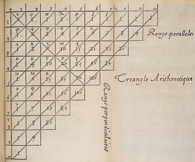
For example, \[ {2 \choose 1} = {1 \choose 1} + {1 \choose 0} = 2 \] and \[ {3 \choose 2} = {2 \choose 2} + {2 \choose 1} = 3. \] Pascal organized these numbers into the table shown in Figure 2.6, which has come to be known as Pascal’s triangle.

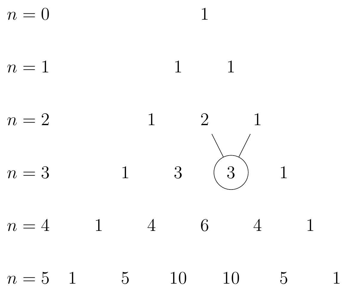
However, the modern Pascal’s triangle is drawn a bit differently, as illustrated in Figure 2.7. Each row contains the binomial coefficients \(n \choose k\) for \(k=0, 1, \dots, n\). For example, the circled value in Figure 2.7 corresponds to \({3 \choose 2}\).

Furthermore, each value can be obtained by adding the two values from the previous row. But this is just Equation 2.5 in words!

Pascal was not the first person to discover the triangle that now bears his name—at least in the Western world. The Persian poet Omar Khayyam (1048-1131) popularized the triangle, and it is still known as “Khayyam’s triangle” (مثلث خیام) in Iran today.

Figure 2.8 shows the triangle as it appeared in a Chinese mathematics text from 1303, Jade Mirror of the Four Unknowns (四元玉鑒). In the Chinese-speaking world, the triangle is known as “Yang Hui’s triangle” (杨辉三角) after the mathematician Yang Hui (1238-1298).

Pascal was not even the first European to discover the triangle, as it had appeared earlier in the works of Cardano. Thus, “Pascal’s triangle” is an example of “Stigler’s Law of Eponymy” (named for the statistician Stephen Stigler), which states that no scientific discovery is named after its original discoverer.

Figure 2.7: Modern version of Pascal’s triangle.

Figure 2.8: Chinese version of Pascal’s triangle.

2.4 Exercises

Exercise 2.1 (Number of events in a finite sample space)

Consider a sample space with three possible outcomes. That is, \[ \Omega = \{ a, b, c \}. \] List all of the possible events. How many are there?
Argue that for any sample space \(\Omega\) with a finite number of outcomes, the number of events is \(2^{|\Omega|}\).

Exercise 2.2 (Round robin tournament) In a round robin tournament, every team plays every other team once. If there are \(n\) teams, how many total games are played? Express your answer as a binomial coefficient.

Exercise 2.3 (Trying keys at random) A friend asked you to house-sit while she is on vacation. She gave you a keychain with \(n\) keys, but she forgot to tell you which key was the one to her apartment. You decide to try keys at random until you find the right one.

If you discard keys that do not work, what is the probability that you will open her apartment on the \(k\)th try?
What is the probability if you do not discard keys that do not work?

Exercise 2.4 (Each side comes up exactly once) The frequentist interpretation of probability says that if we were to toss a fair die many, many times, then each of the six sides should come up about \(1/6\) of the time.

Suppose we toss a fair die six times. Is it likely that each side will come up exactly once? Calculate the probability.

Exercise 2.5 (Elevator stops) You enter an elevator on the first floor of a 15-floor hotel with 3 strangers. You are staying on the 10th floor. If the other 3 people in the elevator are equally to be staying on floors 2 to 15, independently of one another, what is…

the probability that the elevator will stop three times before arriving at your floor? (Ugh!)
the probability that the elevator will not stop at all before arriving at your floor? (Yay!)

Exercise 2.6 (Probability of a Yarborough) In the card game bridge, each player is dealt a hand of 13 cards from a shuffled deck of 52 cards. In the 19th century, the Earl of Yarborough was known to offer 1000-to-1 odds that a bridge hand would contain at least one card that was ten or higher. As a result, a hand that has no cards higher than nine is called a Yarborough. What is the probability of a Yarborough? Was the Earl’s bet favorable or unfavorable to him?

Exercise 2.7 (Rooks on a chessboard) In chess, a rook is able to capture any piece that is in the same row or column. If \(8\) rooks are placed at random on a standard chessboard (\(8\times 8\)), what is the probability that no rook can capture any other?

Exercise 2.8 (Hash collisions) In computer science, a hash table is a data structure for storing information so that it can be accessed quickly. A hash table contains \(n\) “addresses” where data can be stored. For simplicity, we will assume that these addresses are labeled \(1, 2, \dots, n\).

For example, consider an American company that maintains employee records. Each employee is uniquely identified by their Social Security Number (SSN) \(s\), which is then “hashed” by a hash function \(h(s)\), which returns a number \(1, 2, \dots, n\). The data for that employee is then stored at that address. A hash function always returns the same address for a given SSN \(s\), but over many SSNs, a hash function behaves like a random number generator, with each number \(1, 2, \dots, n\) equally likely.

One problem with hash tables is the potential for a hash collision: when two employees have different SSNs \(s_1\) and \(s_2\) that are hashed to the same address, \(h(s_1) = h(s_2)\). Since we can only store one employee’s records at that address, alternative approaches are required.

For a hash table with \(k\) records and \(n\) addresses, calculate the probability of a hash collision.

Exercise 2.9 (Probability of a four-of-a-kind) In poker, what is the probability of a four-of-a-kind (four cards of the same rank, plus one additional card)? Calculate this probability in two ways:

counting hands where order matters
counting hands where order doesn’t matter

Exercise 2.10 (Probability of \(k\) heads in \(n\) tosses) Show that the probability of observing exactly \(k\) heads in \(n\) tosses of a fair coin is \[ P(\text{exactly } k \text{ heads in } n \text{ flips}) = \frac{{n \choose k}}{2^n}. \]

Exercise 2.11 (Combinatorics of DNA) The evolutionary biologist Richard Dawkins (1998) opened his book Unweaving the Rainbow with the following poetic passage:

We are going to die, and that makes us the lucky ones. Most people are never going to die because they are never going to be born. The potential people who could have been here in my place but who will in fact never see the light of day outnumber the sand grains of Arabia. Certainly those unborn ghosts include greater poets than Keats, greater scientists than Newton. We know this because the set of possible people allowed by our DNA so massively outnumbers the set of actual people. In the teeth of these stupefying odds it is you and I, in our ordinariness, that are here.

In this exercise, we will determine these “stupefying odds” by counting the number of possible people. The human genome consists of approximately \(3.1 \times 10^9\) bases. Each base is one of four molecules: adenine (A), thymine (T), guanine (G), or cytosine (C). How many possible genomes are there?

Exercise 2.12 (Combinatorics of proteins) DNA is turned into protein via the central dogma of biology. It is first transcribed into messenger RNA, then translated into amino acids via the process shown in Figure 2.9. Amino acids are the building blocks of all proteins.

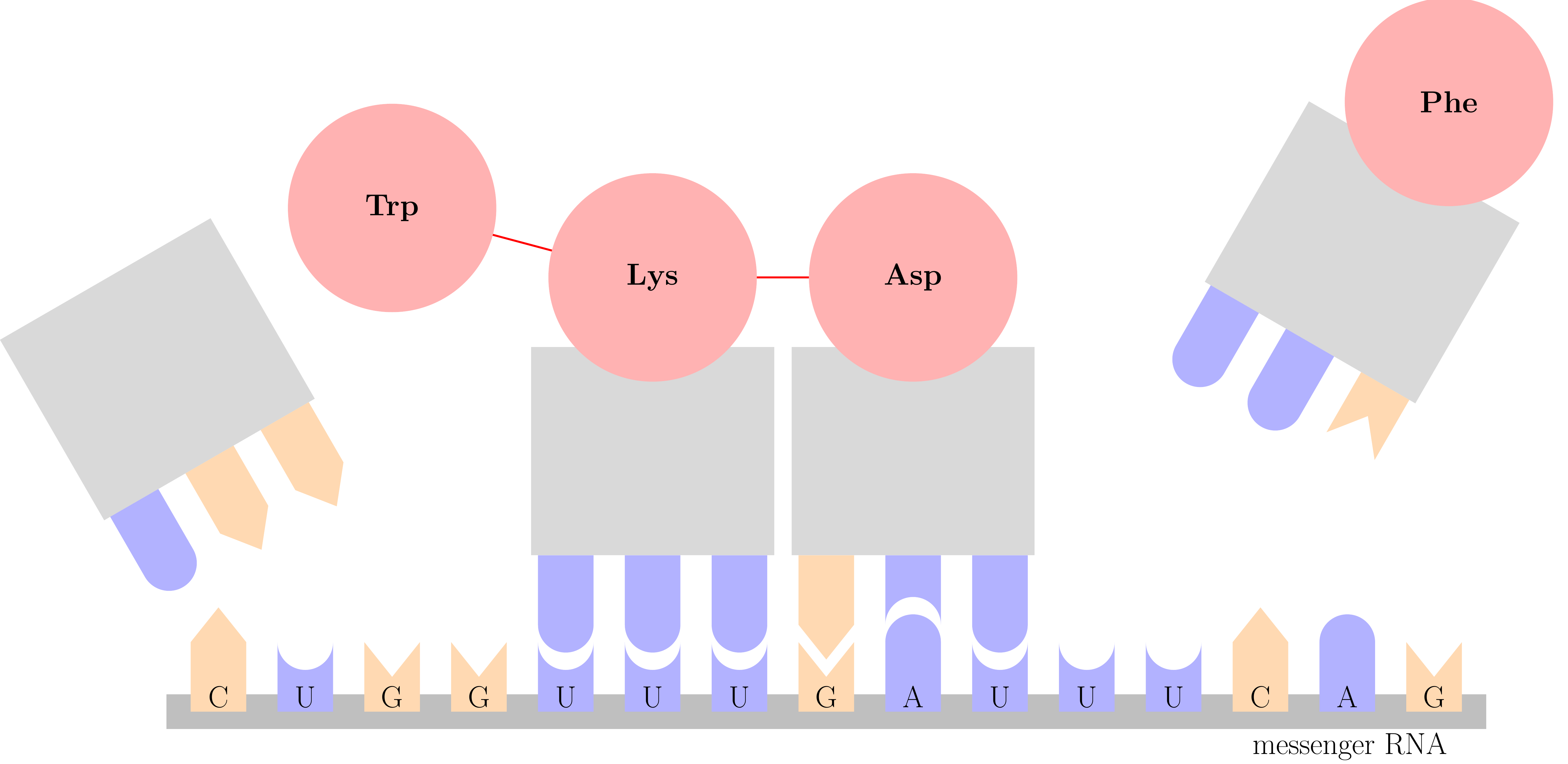
Figure 2.9: RNA is translated to amino acids when tRNA molecules containing an amino acid attach to the mRNA.

Notice that it takes three bases to code for each amino acid. There are 20 different amino acids in total. The order of the bases matters, so UGG codes for tryptophan, while GGU would code for glycine.

Using counting, explain why three bases are needed to code for amino acids. (Why would two bases not be enough?)
Before biologists discovered translation, the physicist George Gamow suggested that the same three bases, in any order, code for the same amino acid. That is, under Gamow’s proposal, UGG, GGU, and GUG would all code for the same amino acid. How many distinct amino acids could be represented under Gamow’s proposal?

In some sense, Gamow’s solution was more mathematically elegant than nature’s solution. For a survey of this and other proposals for the genetic code, see Hayes (1998).

Exercise 2.13 (Galileo’s problem) The Grand Duke of Tuscany observed that rolling three fair six-sided dice resulted in a sum of 10 more often than a sum of 9. Since he counted exactly six ways to obtain each sum, he was puzzled. He consulted one of the finest minds in Tuscany, the astronomer and physicist Galileo Galilei, provided a satisfactory explanation. Your task is to reconstruct Galileo’s argument.

If the order in which the three numbers are rolled does not matter, how many possible outcomes are there? How many of these yield a sum of 9? How many yield a sum of 10?
If the order in which the three numbers are rolled does matter, how many possible outcomes are there? How many of these yield a sum of 9? How many yield a sum of 10?
What is the probability of rolling three numbers that sum to 9? What about the probability of rolling three numbers that sum to 10? Which of the previous parts was most useful in answering these questions? Why?
In words, explain the flaw in the Duke’s reasoning.

Exercise 2.14 (Number of integer solutions) How many different integer solutions \((x_1, x_2, \dots, x_k)\) are there to the equation \[ x_1 + x_2 + \dots + x_k = n \] if

the \(x_i\)s are all non-negative? (Hint: Which of the four cases of Table 2.1 does this correspond to?)
the \(x_i\)s are all positive? Assume for this part that \(k \leq n\) so that there is at least one solution. (Hint: If the \(x_i\)s are positive, then you can start by assigning \(1\) to each \(x_i\), and then the problem reduces to part a above.)

Exercise 2.15 (Number of bootstrap samples) In statistics, it is useful to generate new data sets with similar properties to an original data set. For example, suppose we have data \(w_1, w_2, \dots, w_n\) on \(n\) subjects, representing their weights (in kilograms). For simplicity, we will assume that \(w_1, w_2, \dots, w_n\) are all distinct.

One popular way to generate a new data set with similar properties to the original data set is the bootstrap. (Efron 1979) In the bootstrap, we sample with replacement from the original data. So for example, if \(n=3\) and \(w_1=62\), \(w_2=75\), and \(w_3=69\), then possible bootstrap data sets include

\(w_1^* = 69, w_2^* = 62, w_3^* = 69\)
\(w_1^* = 69, w_2^* = 75, w_3^* = 62\)
\(w_1^* = 75, w_2^* = 75, w_3^* = 75\)
\(w_1^* = 69, w_2^* = 69, w_3^* = 62\)

Notice that the bootstrap always generates a new data set that is the same size as the original data set, but values may be repeated.

What is the probability that the bootstrap generates a data set that consists of the same \(n\) values as the original data set (except possibly in a different order)?
In statistics, the order of the data is often arbitrary, so the bootstrap data sets 1 and 4 above are essentially the same, since both consist of two \(69\)s and one \(62\). How many distinct bootstrap samples are there, if we ignore order? Are these bootstrap samples equally likely?

Exercise 2.16 (Ordering the four ways of counting) Table 2.1 shows the four ways of interpreting the question, “How many ways are there to pick \(k\) items from \(n\) (unique) items?” Order these values from largest to smallest, and prove your answer.

Exercise 2.17 (Problem of points, general case) Recall the problem of points (Example 1.10). Now suppose the players are playing to \(n\) points, but the game is interrupted when Player A has \(a\) points and Player B has \(b\) points. Give a general formula for a fair way to divide the stakes in terms of \(a\), \(b\), and \(n\). Your answer should involve sums of binomial coefficients.

Remark: Pascal invented his famous triangle to calculate these binomial coefficients efficiently.

2.4.1 Combinatorial Identities

Exercise 2.18 (Choosing the complement) Prove the following identity in two ways: by algebra and by counting in two ways.

\[ {{n}\choose{k}} = {{n}\choose{n-k}}. \tag{2.6}\]

Exercise 2.19 (Vandermonde’s identity) Prove Vandermonde’s identity by counting in two ways.

\[ {{m+n}\choose{k}} = \sum_{j=0}^k {{m}\choose{j}} {{n}\choose{k-j}} . \tag{2.7}\]

We will use this identity later in Example 10.4.

Exercise 2.20 (Hockey stick identity) Prove the hockey stick identity: \[ \sum_{m=r}^{n} \binom{m}{r} = \binom{n+1}{r+1}. \] Try doing this in several ways:

by counting in two ways (Hint: Consider choosing \(r+1\) numbers from the set \(\{ 1, 2, \dots, n+1 \}\). Now, what if you first choose the largest number and then choose the remaining \(r\) numbers?)
by repeatedly applying Pascal’s identity (Proposition 2.6)

If you sketch the above identity on Pascal’s triangle, you will see why it is called the “hockey stick identity.”

We will use this identity later in Example 30.1.

Exercise 2.21 (Binomial theorem) Give a combinatorial argument for the binomial theorem: \[ (x + y)^n = \sum_{k=0}^n {n \choose k} x^k y^{n-k}. \]

Hint: Expand the left-hand side, and argue that the number of terms of that reduce to \(x^k y^{n-k}\) is \({n \choose k}\).

Exercise 2.22 (Sum of first \(n\) positive integers) According to a famous legend, the future mathematician Carl Friedrich Gauss was assigned by his schoolmaster to add the numbers from \(1\) to \(100\). The schoolmaster was astonished when the young Gauss finished the task within a few minutes. Gauss realized that he could pair off the numbers—the smallest with the largest, the second-smallest with the second-largest, and so on—so that each pair had a sum of \(101\): \[ \begin{align} 1 + 2 + \dots + 99 + 100 &= (\underbrace{1 + 100}_{101}) + (\underbrace{2 + 99}_{101}) + \dots + (\underbrace{50 + 51}_{101}) \\ &= 50 \cdot 101 \\ &= 5050. \end{align} \] Hayes (2006) provides the history of this legend.

Derive a general formula for the sum of the first \(n\) positive integers. A simple approach is to count the number of games in a round robin tournament (Exercise 2.2) in two ways, thereby showing that \[ 1 + 2 + \dots + n = \sum_{k=1}^n k = \binom{n+1}{2} = \frac{(n+1)n}{2}. \]

This identity is also useful in probability. We will use it later in Exercise 9.7.

Exercise 2.23 (Picking committees with officers) Prove the following identities by counting in two ways.

\(\displaystyle \sum_{k=0}^n \binom{n}{k} = 2^n\)
\(\displaystyle \sum_{k=1}^n k \binom{n}{k} = n 2^{n-1}\)
\(\displaystyle \sum_{k=1}^n k^2 \binom{n}{k} = n(n+1) 2^{n-2}\)
\(\displaystyle \sum_{k=1}^n k^3 \binom{n}{k} = n^2(n+3) 2^{n-3}\)

(Hint: Count the number of committees with 0, 1, 2, and 3 officers, respectively, where the same person can occupy the same office.)