46 Hypothesis Testing
$$
$$
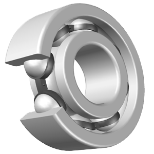
For example, consider a company that manufactures engine ball bearings, such as the one shown in Figure 46.1. The diameter of the inner ring must be manufactured to a high degree of precision to ensure that a shaft or axle fits into the ball bearing.
One model that the company manufactures is designed to have an inner diameter of exactly \(10.00\text{mm}\). However, the manufacturing process is not perfectly precise, so under normal manufacturing conditions, the actual inner diameter of the ball bearings are normally distributed around \(10.00\text{mm}\), with a standard deviation of \(0.03\text{mm}\). That is, the inner diameters \(X_i\) are i.i.d. \(\textrm{Normal}(\mu= 10.00, \sigma^2= 0.03^2)\).
The quality control department at the company measures 5 ball bearings each day to ensure that the inner diameter remains within specifications. One day, the quality control department measures \[ X_1 = 10.06, X_2 = 10.07, X_3 = 9.98, X_4 = 10.02, X_5 = 10.09. \]
If \(\mu\) represents the actual target inner diameter of the ball bearings that day, we know that we can estimate \(\mu\) by the maximum likelihood estimator \[ \bar X = 10.044. \]
However, the company is less interested in estimating \(\mu\) than in determining whether \(\mu\) has deviated from the target value of \(10.00\text{mm}\), in which case the manufacturing process may need to be adjusted. This is a classic application of hypothesis testing.
46.1 The \(z\)-test
The goal of hypothesis testing is to determine whether the data provides evidence for or against a null hypothesis. In the ball bearing example, the null hypothesis is that the process is “in control”; that is, the true inner diameter of the ball bearings is \(10.00\text{mm}\). We denote this null hypothesis by: \[ H_0 : \mu = 10.00 \]
However, we observed that the average inner diameter of 5 ball bearings manufactured on that day was \(\bar X = 10.044\text{mm}\). Although this differs from the target diameter of \(10.00\text{mm}\), this may simply have been an unlucky batch rather than indicating a problem in the manufacturing process. Can we chalk up this difference to chance, or does this data provide evidence against the null hypothesis?
To answer this question, we quantify how likely it is to observe \(\bar X = 10.044\) if in fact \(\mu = 10.00\). If it is very unlikely, then we conclude that this did not happen by chance and reject the null hypothesis.
How low does the p-value need to be before we reject the null hypothesis? Typically, statisticians use a threshold of 5%. If the p-value is below 5%, then they reject the null hypothesis; otherwise, they do not reject it.
46.2 The \(t\)-test
There is one major limitation of the \(z\)-test: it requires knowing the population variance \(\sigma^2\). While this may be reasonable in quality control applications, where this population variance is known from years of manufacturing, this is not the case for most applications.
For example, Mackowiak, Wasserman, and Levine (1992) wanted to evaluate whether the average human body temperature really is \(98.6^\circ\text{F}\), a number that originated with the 19th century physician Carl Reinhold August Wunderlich. To evaluate Wunderlich’s reference point, Mackowiak, Wasserman, and Levine (1992) measured the body temperatures (in \({}^\circ\text{F}\)) of \(n=130\) patients; their data is reproduced below.
Mackowiak, Wasserman, and Levine (1992) were interested in testing the null hypothesis \[ H_0: \mu = 98.6. \]
Human body temperatures are approximately normally distributed, as the above histogram shows. However, we do not know the population variance \(\sigma^2\) of human body temperatures. Therefore, we cannot use the test statistic \[ Z = \frac{\bar{X} - \mu_0}{\sqrt{\sigma^2/n}} \tag{46.1}\] to test this hypothesis.
One natural idea is to replace \(\sigma^2\) with an estimate, such as the sample variance \(S^2\) (Equation 32.13). That is, we can instead use the test statistic \[ T = \frac{\bar X - \mu_0}{\sqrt{S^2 / n}}. \tag{46.2}\]
However, because of the additional variability from \(S^2\), Equation 46.2 will not follow a standard normal distribution. Instead, it follows a new distribution, which we derive now.
First, we will rewrite Equation 46.2 in a more abstract and general form: \[ T = \frac{\frac{\bar X - \mu}{\sqrt{\sigma^2/n}}}{\sqrt{\frac{S^2}{\sigma^2}}} = \frac{Z}{\sqrt{W / (n-1)}}. \tag{46.3}\] The numerator is simply a standard normal random variable \(Z\), while the denominator is the square root of a \(\chi^2_{n-1}\) random variable \(W\) divided by \((n-1)\). This follows from Theorem 45.3, which says that \[ (n-1)\frac{S^2}{\sigma^2} \sim \chi^2_{n-1}. \] Furthermore, by Theorem 44.2, we know that \(\bar X\) and \(S^2\) are independent, so \(Z\) (which only depends on \(\bar X\)) and \(W\) (which only depends on \(S^2\)) are also independent.
The upshot of this discussion is that to find the distribution of Equation 46.2, we need to find the distribution of a random variable of the following form.
Notice that the statistic Equation 46.2 corresponds to Definition 46.1 with \(k = n - 1\). However, the \(t\) distribution arises in other contexts besides this one; see Exercise 45.2 for an example.
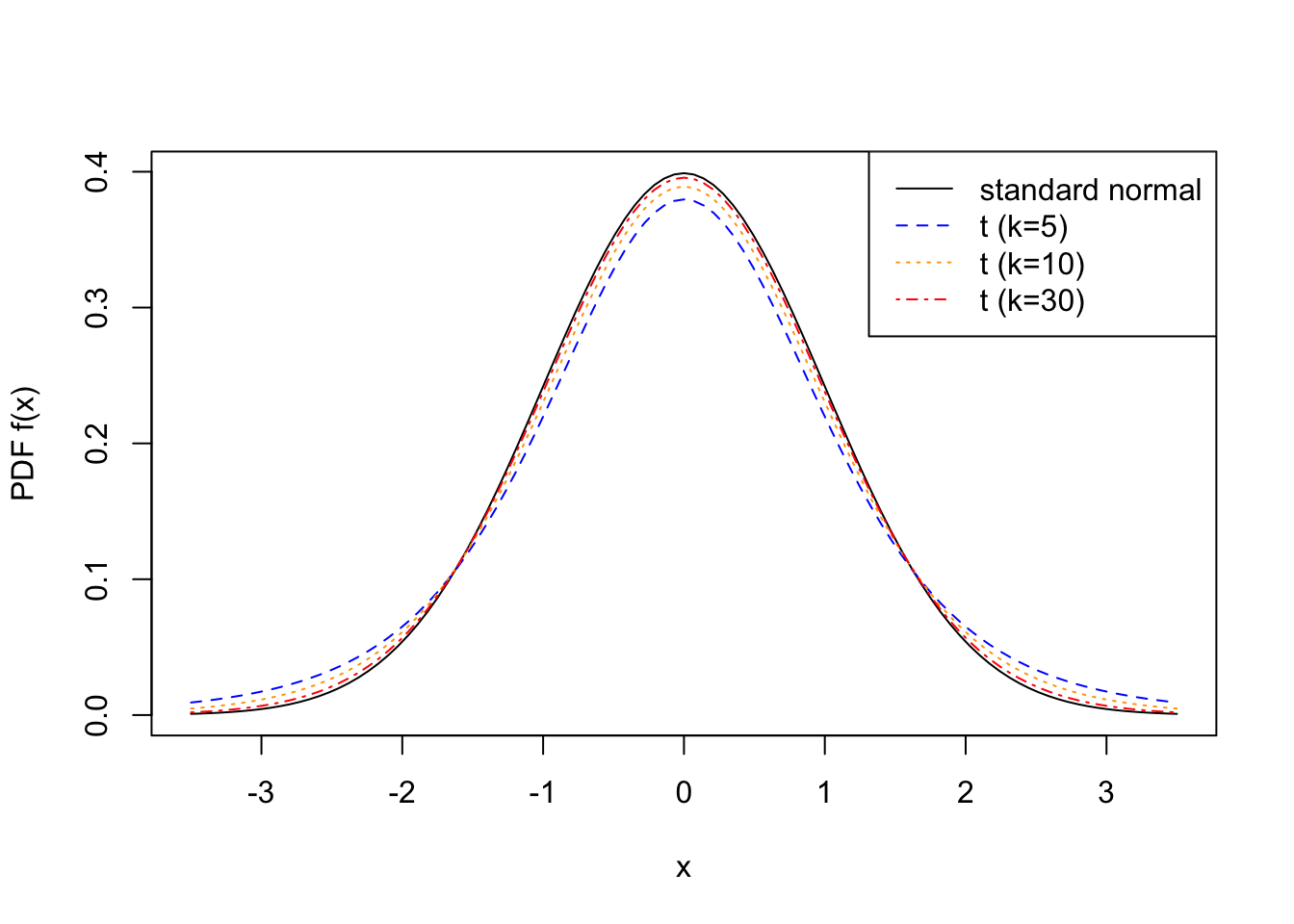
Next, we derive the PDF of the \(t\) distribution.
The PDF Equation 46.5 is graphed in Figure 46.2 for different degrees of freedom \(k\). Notice that, like the standard normal distribution, the \(t\) distribution is symmetric around zero. However, it has “heavier” tails—that is, more probability in the tails.
In practice, we rarely need the formula for the PDF (Equation 46.5), since we can simply use functions like pt(..., df) in R to evaluate probabilities under a \(t\) distribution. However, the formula for the PDF allows us to describe theoretically just how much heavier the tails of the \(t\) distribution are. \[
\begin{align}
f(x) \propto \left(1 + \frac{x^2}{k} \right)^{-(k+1) / 2} &\sim \frac{k^{(k+1)/2}}{x^{k+1}} & \text{(as $x \to \infty)$.}
\end{align}
\] Ignoring the numerator (which is just a constant), the decay is polynomial (\(1 / x^{k+1}\)), which is much slower than the super-exponential decay (\(e^{-x^2}\)) of the normal distribution.
We can use the \(t\) distribution to carry out the hypothesis test for the mean body temperature example.
If we had instead used the standard normal distribution to calculate the p-value, we would have obtained a smaller probability.
This makes sense because, as Figure 46.2 shows, the \(t\) distribution has heavier tails than the standard normal distribution. One way to see why is to compare the original test statistics \(Z\) (Equation 46.1) and \(T\) (Equation 46.2); extra variability is introduced when \(\sigma^2\) is replaced by \(S^2\).
Figure 46.2 illustrates another phenomenon: the \(t\) distribution approaches the standard normal distribution as the degrees of freedom \(k\) increases. Again, the test statistic provides some insight here; as \(n \to\infty\), \(S^2\) is very close to \(\sigma^2\), so there is essentially no difference between using \(S^2\) or \(\sigma^2\) when \(n\) is large. The next proposition formalizes this intuition.
The practical consequence of Proposition 46.2 is that there is little difference between using the \(z\)-test or the \(t\)-test when \(n\) is large.
46.3 Asymptotic Tests
All of the tests above assumed that the \(X_1, \dots, X_n\) were i.i.d. normal. What do we do if the data are not normal? It is no longer feasible to obtain an exact p-value, but an approximate p-value is still within reach, thanks to the Central Limit Theorem (Theorem 36.1).
For example, recall the skew die example (Example 29.4) from the very beginning of our foray into statistical inference.
Example 46.3 is unsatisfying because we only examined sixes, when the skew die could favor any side. Suppose that in the \(n=25\) rolls, we observed the number of times each side came up: \[ \vec X = (1, 7, 6, 4, 0, 7). \] Then, \(\vec X\) follows a \(\text{Multinomial}(n=25, \vec p)\) distribution (Definition 43.4), and we want to test \[ H_0: \vec p = (\frac{1}{6}, \frac{1}{6}, \frac{1}{6}, \frac{1}{6}, \frac{1}{6}, \frac{1}{6}). \]
Here is a test statistic that takes into account all six sides of the die. We can compare the observed count \(X_j\) to the expected count \(n p_j\), normalizing by the expected count (since the difference will naturally be larger for categories with a higher count), then aggregate this difference across the categories. That is, \[ W = \sum_{j=1}^k \frac{(X_j - np_j)^2}{np_j}. \tag{46.6}\]
Large values of \(W\) would imply that \(\vec p\) is not a good model for the data.
To determine how large \(W\) needs to be to reject the null hypothesis, we need to know the distribution of \(W\). The exact distribution is impractical to derive, but an approximate distribution is possible with the help of the Multivariate Central Limit Theorem (Theorem 44.3).
Now, let’s apply Proposition 46.3 to the dice data. We calculate the test statistic and compare it to the \(\chi^2_5\) distribution, as predicted by theory.
The p-value is \(0.047\), which is less than \(0.05\), so we reject the null hypothesis. When we consider all six sides, there is enough evidence conclude that the skew die is not fair. Not only are there too many sixes, but there are also too many twos and threes; when we combine all of this evidence, it is no longer reasonable to assume that the skew die is fair.
It is important to remember that the p-value above is approximate because it relied on the Multivariate Central Limit Theorem. To see how accurate it is, it is useful to conduct a simulation study. Let’s compare the simulated distribution of \(W\) under the null hypothesis, with the \(\chi^2_5\) distribution predicted by Proposition 46.3.
The approximation is surprisingly accurate, even when \(n\) is just \(25\).
46.4 Exercises
Exercise 46.1 When simulating basketball games, some people a Gaussian random number generator (a random sample from \(\text{Normal}(0,1)\)) to assign a “heat index” to each player. For example, if Steph Curry’s field goal probability is known to be \(0.471\) with standard deviation \(0.105\), and the random number generator outputs \(0.453\) for Steph, then for that day, Steph will have a \(+0.453\) SD performance; i.e., his shooting percentage that day will be \[ 0.471 + 0.453 \cdot 0.105 = 0.519. \] This updated percentage will be used for Steph in simulating games that day.
One day, you are simulating games involving \(232\) players, and the \(232\) numbers generated have mean \(0.31\). Is there enough evidence to suspect that our Gaussian random number generator is not sampling from a mean \(0\) distribution?
Exercise 46.2 What if we repeat the same process in Exercise 46.1, but instead of using a Gaussian random number generator, we instead sample from \(\text{Uniform}(-2,2)\) in order to assign heat indices to the players?
Suppose we generate \(232\) numbers, and they have mean \(0.31\). If \(X_1, \dots, X_{232}\) represent a random sample of size \(232\) from \(\text{Uniform}(-2,2)\), we cannot directly use the \(z\)-test as we are not sampling from a normal distribution. However, it turns out we can, by using the Central Limit Theorem.
- What is the approximate distribution of \(\bar{X}\), according to the Central Limit Theorem?
- Use the result to determine the p-value of the observed outcome. Is there enough evidence to suspect that our uniform random number generator is not sampling from a mean \(0\) distribution?
Exercise 46.3 Stout beers are flavored with the flowers of the plant humulus lupulus, widely known as hops. The trademark bitter flavor comes from resins, a semisolid substance from the glands of the hops.
A particular brewery wants to the proportion of soft resins to be 8.5%. In a batch of \(12\) samples, the brewmaster gets the proportion of soft resins \[ 7.8, 8.5, 8.6, 8.2, 8.0, 8.4, 8.2, 7.7, 8.2, 8.2, 8.1, 8.0 \] Is there enough evidence to conclude that the machine is producing beer with the proportion of soft resins not equal to 8.5%?
Exercise 46.4 (Alternative derivation of the \(t\) distribution) Derive the joint distribution of \(T = \frac{Z}{\sqrt{W / (n-1)}}\) and \(U = W / (n-1)\).
Use this joint distribution to derive the PDF of \(T\).
Exercise 46.5 (Two-sample \(t\)-test) Let \(X_1, \dots, X_m\) be i.i.d. \(\text{Normal}(\mu_1, \sigma^2)\) and \(Y_1, \dots, Y_n\) be i.i.d. \(\text{Normal}(\mu_2, \sigma^2)\).
Under the null hypothesis that \(\mu_1 = \mu_2\), we are in the situation of Exercise 45.2. Using the results from that exercise, derive the distribution of the test statistic
\[ T = \frac{\bar X - \bar Y}{\sqrt{\frac{S_{\text{pooled}}^2}{m} + \frac{S_{\text{pooled}}^2}{n}}}. \]
The hypothesis test based on this test statistic is known as the two-sample \(t\)-test.
Exercise 46.6 (Test for the variance) Let \(X_1, \dots, X_n\) be i.i.d. \(\text{Normal}(\mu, \sigma^2)\). Describe a test of \[ H_0: \sigma^2 = \sigma_0^2. \] For what values of \(X_1, \dots, X_n\) would you reject the null hypothesis?
Hint: Use the result of Theorem 45.3.