1 Classical Definition of Probability
$$
$$
One summer morning in Los Angeles, a blonde-haired woman with a ponytail snatched another woman’s handbag. She fled the scene in a yellow car driven by a Black man with a beard and a mustache. Four days later, a police officer visited a house with a yellow car parked outside, occupied by a woman with blonde hair in a ponytail and a bearded and mustachioed Black man. Could this have been the couple that committed the crime?
This scenario is not hypothetical; it was the subject of the court case People v. Collins. The prosecution contended that the chance of a random couple having those exact attributes was so small (one in 12 million) that the accused must be the actual culprits. The argument compelled the jurors, who reached a guilty verdict. The case was then appealed to the California Supreme Court, where the defense argued that the relevant probability was not the chance of a random couple having these attributes, but rather the chance that at least two couples with these same attributes exist. After all, if there were many couples that shared these attributes, then the prosecution could not conclude beyond a reasonable doubt that the accused was the guilty party. For a city the size of Los Angeles, the defense computed this latter probability to over 40% (even while using the prosecution’s questionable and unfavorable assumptions). Persuaded by the defense’s argument, the court felt there was insufficient evidence to implicate the accused and overturned the guilty verdict.
One feature of the above scenario, common to many real-world situations, is that a decision needs to be made under uncertainty. The court needs to decide whether the couple is guilty or not, but it cannot be sure that this couple is the same as the one at the scene of the crime. When uncertainty is involved, it is easy to slip into fallacious reasoning, as the prosecution did in the original trial.
Probability theory, the subject of this book, is the mathematical study of uncertainty. By learning the rules of probability, you will improve your ability to quantify, and thereby make decisions under, uncertainty. These skills are applicable not only in law, but also in a wide range of other fields, including:
- Economics and finance: Prices of assets, such as stocks and houses, fluctuate daily, and probability models are used to decide when to buy and sell assets.
- Biology and medicine: In genetics, probability helps predict traits and calculate the risk of hereditary diseases. In medicine, probabilistic models inform diagnosis and personalized medicine strategies.
- Physical sciences and engineering: At a fundamental level, thermodynamics and quantum mechanics are inherently probabilistic theories. In applied fields, engineers use probability to design reliable systems, model climate dynamics, and optimize performance in uncertain environments.
- Computer science and machine learning: Randomized algorithms like quicksort or Monte Carlo simulations exploit randomness to improve efficiency and tackle computationally hard problems. Machine learning models, from Bayesian networks to deep learning, rely on probabilistic reasoning to both learn patterns and make predictions from data. For example, large language models use probabilities to both learn language and decide how best to respond to our prompts.
- Statistics: More generally, probability underpins the tools we use to draw inferences from data. Through statistics, probability indirectly supports nearly every field, including the social sciences and the digital humanities.
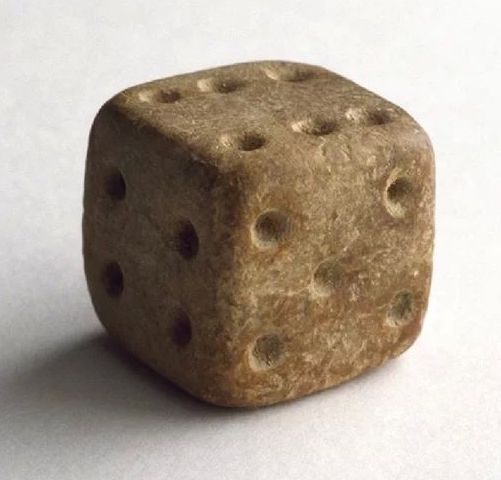
We will encounter real applications of probability to each of the above fields throughout this book. However, we start by examining the more frivolous endeavor for which probability theory was first invented: games. Although games of chance are as old as civilization itself (Figure 1.1 shows a 4,000-year-old die that looks surprisingly modern), it was not until the 16th century that the games were analyzed systematically.
1.1 A Need for a Mathematical Framework
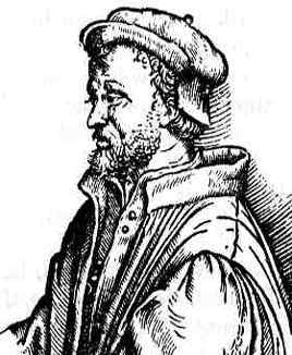
One of the first people to analyze games of chance was the Italian doctor, mathematician, and gambler Gerolamo Cardano. Cardano was the first European to use negative numbers (which were already widely used in China, India, and the Islamic world). He was the first to publish the cubic formula and quartic formula, analogues of the famous quadratic formula for polynomials of higher degree. Cardano combined his loves of gambling and mathematics in his 1564 book, Liber de ludo aleae (“Book on Games of Chance”), which contained problems like the following.
Cardano’s solution may seem plausible at first, but his reasoning is clearly flawed. By the same logic, if the die were rolled \(k=6\) times, the probability of seeing at least one six would be \(6 \times 1/6 = 100\%\). But even with \(k=6\) throws, we are not guaranteed to see a six. In fact, if every reader of this book were to roll a six-sided die \(k=6\) times, about a third would not see any sixes. In Example 4.1, we will see that \(k=3\) throws gives only a \(42.1\%\) chance of seeing at least one six, and \(k=4\) throws are required to achieve a better than \(50\%\) chance.
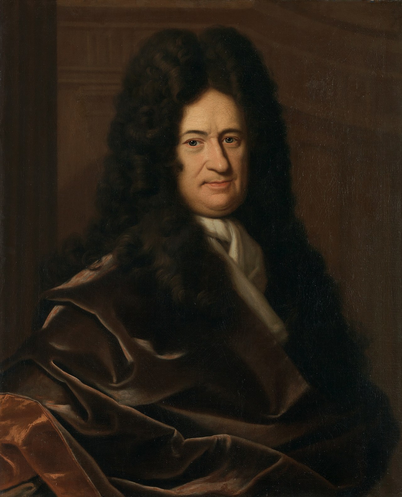
Gottfried Leibniz was a German polymath who may be best remembered for his dispute with Isaac Newton over who invented calculus first. However, he also made groundbreaking contributions to library science, philosophy, and theology. In fact, his philosophy was caricatured by Voltaire through the character Dr. Pangloss in the novel Candide. Leibniz also dabbled in probability theory. In his Opera Omnia (“Complete Works”), he studied the following question.
Leibniz’s solution is incorrect, and we will see in Solution 1.1 that an eleven is actually twice as likely as a twelve.
The French physicist and mathematician Jean le Rond d’Alembert is best remembered for discovering and solving the wave equation, a partial differential equation that describes how sound and light waves propagate. He also made other contributions to mathematics, including the ratio test for infinite series. In his 1754 article Croix ou Pile (“Heads or Tails”), he studied the following probability problem.
D’Alembert’s solution is also mistaken, as we will see in Solution 1.2.
Our reason for recounting these historical blunders is threefold:
Probability requires a mathematical foundation. If some of the greatest minds computed probabilities incorrectly when relying on intuition, any of us could do the same. By correctly following the mathematical framework laid out in this book, you will be able to avoid the errors of Cardano, Leibniz, and d’Alembert.
These problems are less difficult today because of probability theory. By the end of this chapter, you will be able to correctly reason through the problems that baffled these mathematicians. This is a testament to the success of probability theory over the last 400 years. As Isaac Newton famously said, “If I have seen further, it is by standing on the shoulders of giants.”
But probability is still difficult. If Leibniz, who invented a subject as complex as calculus, could stumble on a basic probability calculation, then any one of us could too. Even with the resources at our disposal today, probability is still a difficult subject, especially on a first pass. As you go through this book, do not be discouraged if concepts seem challenging or counterintuitive at first.
1.2 The Classical Definition of Probability
In order to lay the foundations of probability, we first need to define probability mathematically. Our first definition, based on the ideas of Cardano himself, is called the classical definition of probability. We will develop this definition using the casino game of roulette.
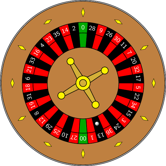
Roulette takes its name from the French word for “little wheel.” True to its name, the game involves tossing a ball into a spinning wheel and making bets about the pocket that the ball will settle in. Figure 1.5 shows an American roulette wheel, which has 38 pockets: 37 pockets labeled 0 to 36 and an additional pocket labeled 00. (Note that a European roulette wheel only has 37 pockets; it lacks the 00 pocket.)
Fyodor Dostoevsky’s novel The Gambler tells the story of a young man’s descent into roulette addiction. He relates the thrill of his first encounter with the game:
At first the proceedings were pure Greek to me. I could only divine and distinguish that stakes were hazarded on numbers, on “odd” or “even,” and on colors…. I began by pulling out fifty gulden, and staking them on “even.” The wheel spun and stopped at 13. I had lost! With a feeling like a sick qualm, as though I would like to make my way out of the crowd and go home, I staked another fifty gulden—this time on the red. The red turned up. Next time I staked the 100 gulden just where they lay—and again the red turned up. Again I staked the whole sum, and again the red turned up. Clutching my 400 gulden, I placed 200 of them on twelve numbers, to see what would come of it. The result was that the croupier paid me out three times my total stake! Thus from 100 gulden my store had grown to 800!
The narrator bets on red, which pays out when the ball lands in a red pocket (see Figure 1.5). Now, we use the classical definition of probability to describe the chances of winning such a bet.
The classical definition of probability considers an experiment with a finite number of possible, equally likely, outcomes. These outcomes make up the sample space of the experiment.
Later, we will see in Chapter 3 that the classical definition cannot be used to analyze many important random phenomena. However, it is sufficient for games like roulette: spins of the roulette wheel can be repeated indefinitely, and the wheel’s symmetry and balanced spin mechanism are carefully designed to ensure that the ball is equally likely to land in any of the 38 pockets.
In the case of our roulette “experiment,” the different possible outcomes are the different pockets the ball may land in, which are depicted in Figure 1.5. These pockets are best identified by their numerical label, and hence we can write our sample space as
\[ \Omega = \{ \textcolor{green}{00}, \textcolor{green}{0}, \textcolor{red}{1}, \textcolor{black}{2}, \textcolor{red}{3}, \dots, \textcolor{red}{34}, \textcolor{black}{35}, \textcolor{red}{36} \}. \]
Having defined the experiment and the sample space, we want to know the probability of some event happening, such as the probability that the ball lands in a red pocket. Any event corresponds to a subset \(A\) of the possible outcomes. For example, the event that the ball lands in a red pocket corresponds to the subset \[ A = \{ \textcolor{red}{1}, \textcolor{red}{3}, \textcolor{red}{5}, \dots, \textcolor{red}{32}, \textcolor{red}{34}, \textcolor{red}{36} \}. \] This motivates the following definition.
Under this setup, Cardano defined the probability of an event to be the ratio of the number of outcomes in the event to the number of outcomes in the sample space: \[ P(A) \overset{\text{def}}{=}\frac{\text{number of outcomes in $A$}}{\text{number of possible outcomes}}. \]
Using the classical definition of probability (Definition 1.3), we can find the probability that a bet on red wins in roulette.
How should we interpret the probability \(P(A)\)? For now, we will adopt the frequentist viewpoint, which says that the probability of an event represents its long-run relative frequency, the proportion of times that the event happens if the experiment is repeated again and again. That is, the frequentist interpretation is
\[ P(A) = \lim_{\text{\# trials} \rightarrow \infty} \frac{\text{\# trials where $A$ happens}}{\text{\# trials}}. \tag{1.1}\]
If we view Example 1.4 through a frequentist lens, the proportion of times that the ball lands on red should get closer and closer to \(18/38 \approx 0.4737\) as the roulette wheel is spun again and again. The code below simulates 1,000 spins of a roulette wheel. Notice that the relative frequency is initially quite far from \(0.4737\) (for instance, after just \(1\) spin, the proportion must be either \(0\) or \(1\)!), but as the number of trials increases, it approaches the probability of \(0.4737\) (represented by the red dashed line).
The next example applies Definition 1.3 to another classic gambling situation: drawing a playing card.
Example 1.5 (Pick a card, any card!) A standard deck of playing cards has \(52\) cards, each of which has one of \(13\) ranks (\(\text{A}\) for ace, \(2\) through \(10\) for numbered cards, \(\text{J}\) for jack, \(\text{Q}\) for queen, and \(\text{K}\) for king) and one of \(4\) suits (\(\clubsuit\) for clubs, \(\textcolor{red}{\diamondsuit}\) for diamonds, \(\spadesuit\) for spades, and \(\textcolor{red}{\heartsuit}\) for hearts). If we randomly select a card from the deck, what is the chance we select a red card?
We are equally likely to select any of the \(52\) cards in our sample space \(\Omega\), which is depicted below in Figure 1.6.
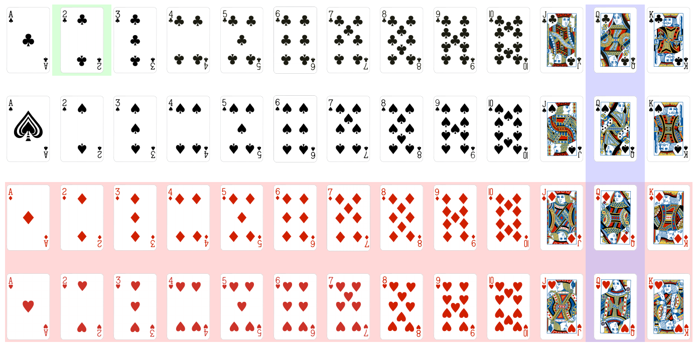
The event of selecting a red card consists of the \(26\) outcomes in Figure 1.6 highlighted in red. Therefore, by the classical definition of probability (Definition 1.3),
\[ P(\textcolor{red}{\text{red}}) = \frac{\textcolor{red}{26}}{52} = 0.50. \]
What about the probability of selecting a queen? This event comprises the \(4\) outcomes in Figure 1.6 highlighted in blue, so \[ P(\textcolor{blue}{\text{queen}}) = \frac{\textcolor{blue}{4}}{52} \approx 0.0769. \]
Since there are \(4\) cards of every rank, we would get the same probability if we asked for, say, a seven.
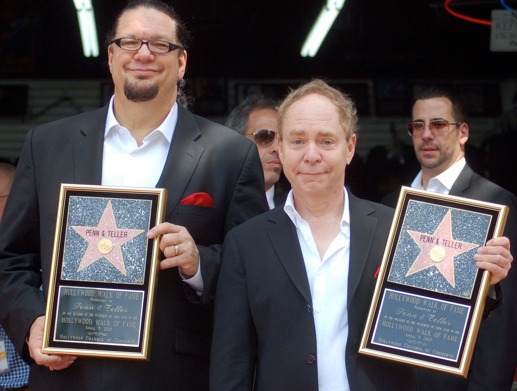
The magicians Penn and Teller (shown at left) are known for “forcing” the Three of Clubs upon unwitting spectators in many of their card tricks. If they truly were selecting a card at random, what is the probability that the spectator would just happen to pick the Three of Clubs?
Since the event of selecting the Three of Clubs consists of just a single outcome (highlighted in green in Figure 1.6),
\[ P(\textcolor{green}{\text{3 of Clubs}}) = \frac{\textcolor{green}{1}}{52} \approx 0.0192. \]
1.3 Applications
The classical definition of probability, although restrictive, already allows us to analyze a wide range of interesting real-world phenomena. Our first example comes from a field whose history and development has been greatly intertwined with probability and statistics: genetics.
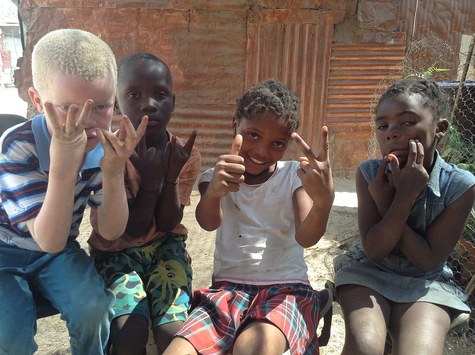
Example 1.6 (Genetic inheritance and albinism)
Albinism is a condition where an individual lacks pigment in their skin and hair. Individuals who exhibit albinism are referred to as “albinos.” For simplicity, we will focus on one genetic cause of albinism: a mutation in the OCA2 gene, which is located on chromosome 15. (Though other genes can also cause albinism, we will ignore those here.)
Gregor Mendel’s 19th-century work on genetics explained how two parents who are not albino can still have an albino child. This happens because every person has two copies of each gene: one inherited from their mother and one from their father.
Each copy of the OCA2 gene can come in one of two versions, which we will represent by letters:
- \(A\): the version of the gene without the mutation
- \(a\): the mutated version that can cause albinism
A person only exhibits albinism if both copies of the OCA2 gene are the mutated version (\(aa\)).
These versions are called “alleles” (pronounced uh-leelz). If a person has at least one copy of the \(A\) allele, then they will not exhibit albinism because the \(A\) allele is “dominant” over the “recessive” \(a\) allele.
Now, imagine two parents, each with one \(A\) and one \(a\) allele (we call them “carriers” of albinism). They are not albino because they each have at least one \(A\) allele, but they can pass the \(a\) allele to their children. Here is how this works.
When a parent produces sperm or egg cells (through a process called meiosis), the two copies of the gene separate, and each cell randomly gets one of the two copies. Hence, when the sperm and egg combine during fertilization, the child gets one copy of the gene from each parent. Empirically, we observe that the \(4\) possible allele combinations, organized in the table below (which is called a “Punnett square”), are equally likely:
| Mother \(\Big\backslash\) Father | \(A\) | \(a\) |
|---|---|---|
| \(A\) | \(AA\) | \(Aa\) |
| \(a\) | \(Aa\) | \(aa\) |
What is the probability of two carrier parents having an albino child? The sample space \(\Omega\) consists of the \(4\) equally likely outcomes in the above table, and the event that the child is albino consists of only the single outcome \(aa\). Therefore, the classical definition of probability (Definition 1.3) tells us that
\[ P(\text{child is albino}) = \frac{1}{4} = 0.25. \]
What does this probability mean? According to the frequentist interpretation, if we look at many offspring of carrier parents, approximately one-quarter of them should be albino.
We now turn to an example where enumerating the sample space is more challenging.
Example 1.7 (Secret Santa)
Four friends participate in a Secret Santa gift exchange. They write their names on slips of paper and place them in a box. The box is then shaken and each friend draws a slip. They then buy a gift for the person whose name they draw.
In a “good” draw, nobody ends up with their own name. Otherwise, the group would need to put the slips back in the box and draw again. What is the probability that the group gets a good draw?
To answer this question, we need to list all the possible outcomes. If we represent each friend by a number (\(1, 2, 3, 4\)), then we can use notation like \[ 2431 \] to denote that friend \(1\) drew friend \(2\), friend \(2\) drew friend \(4\), friend \(3\) drew friend \(3\), and friend \(4\) drew friend \(1\). (In this case, friend \(3\) drew their own name, so this outcome does not belong to the event of interest.)
Now, we can enumerate the \(24\) possible outcomes in our sample space \(\Omega\). These outcomes should be equally likely because the box was shaken, so each friend should be equally likely to draw any slip.
| 1. 1234 | 7. 2134 | 13. 3124 | 19. 4123 |
| 2. 1243 | 8. 2143 | 14. 3142 | 20. 4132 |
| 3. 1324 | 9. 2314 | 15. 3214 | 21. 4213 |
| 4. 1342 | 10. 2341 | 16. 3241 | 22. 4231 |
| 5. 1423 | 11. 2413 | 17. 3412 | 23. 4312 |
| 6. 1432 | 12. 2431 | 18. 3421 | 24. 4321 |
Of these outcomes, the ones corresponding to the event that no friend draws their own name appear in bold. There are \(9\) such outcomes, so \[ P(\text{no one draws their own name}) = \frac{9}{24} = 0.375. \]
What does this probability mean? According to the frequentist interpretation, if the same four friends repeated this tradition for many years, they would achieve a good draw on the first try in approximately \(37.5\%\) of the years.
The next example is a classic brainteaser that caused quite a stir when it was first proposed.
Example 1.8 (The Monty Hall problem)
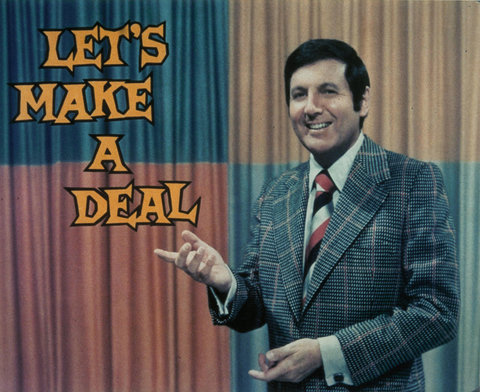
Let’s Make a Deal was a popular game show in the 1960s and 1970s. The host, Monty Hall, would offer contestants a choice between three doors. The contestant could keep whatever was behind the door they chose.

Monty tells the contestant that behind one of the doors is a car, and behind the other two doors are goats. The car is equally likely to be behind any of the three doors, so we can assume that the contestant picks door 1. However, prior to opening door 1, Monty opens one of the other doors to reveal a goat.
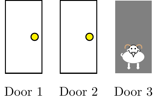
In light of this information, Monty offers the contestant the option to switch from door 1 to door 2. Should the contestant switch?
At first glance, it seems like it should not matter. There are two remaining doors, so why should the car be any more likely to be behind one than the other?
However, surprisingly, the probability of winning the car doubles if the contestant switches! Here is the argument.
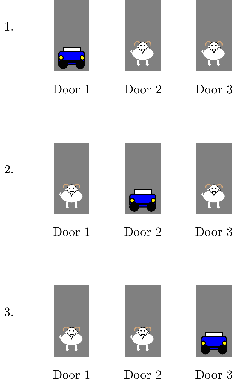
If we assume that the contestant always picks door 1 initially, then the only randomness in the problem comes from which door the car is behind. (We can assume that the contestant always picks door 1 because the analysis would be the same if the contestant picked any other door.) Hence, there are three possible equally likely outcomes that make up the sample space \(\Omega\):
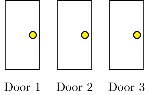
We can now analyze what happens when the contestant switches (or does not).
- Switch: Suppose the contestant switches doors when given the option. If the car is behind door \(1\), then Monty will open one of the other doors, and by switching the contestant ends up with a goat. On the other hand, if the car is behind door \(2\) or door \(3\), then Monty will open the other door with a goat, and by switching, the contestant wins the car. Therefore, the classical definition of probability (Definition 1.3) tells us that
\[ P(\text{win car}) = \frac{2}{3}. \]
- Does not switch: If the contestant does not switch, then they only win if the car is behind the first door. By the classical definition of probability,
\[ P(\text{win car}) = \frac{1}{3}. \]
The Monty Hall problem gained notoriety when Marilyn vos Savant, a columnist for Parade magazine who holds the Guinness Book of World Records for highest recorded IQ, proposed the above solution in 1990. Although it was correct, the magazine received thousands of letters asserting that her solution was wrong, including many from mathematics PhDs. The problem was introduced to a new generation when it was quoted in the 2008 movie 21, based on a true story about MIT students who used probability to beat Las Vegas casinos at Blackjack. Rosenhouse (2009) traces the history and explores extensions of this famous problem.
We now turn to two examples involving fair dice, like the one pictured in Figure 1.1, which further illustrate the classical definition in action. In the first example, we calculate the probability of winning or losing on the first roll (called the come-out roll) in the popular casino game craps.
A brief introduction to craps
Craps is a casino game played by rolling a pair of fair, six-sided dice. In each round, one person (the “shooter”) rolls the dice, while gamblers around the table place bets on the results of those rolls.
Each round consists of two phases:
- In the come-out roll, the shooter wins if a 7 or 11 is rolled and loses if a 2, 3, or 12 is rolled, in which case the round ends. Otherwise, the number that is rolled becomes the point, and the round proceeds to the second phase.
- In the second phase, the shooter repeatedly rolls the dice until either the point or a 7 is rolled again. If the point is rolled first, then the shooter wins; if the 7 is rolled first, then the shooter loses.
The two most common bets that players make in craps are that the shooter will win (called a pass line bet) or that the shooter will lose (called a don’t pass bet).
Example 1.9 (Probability of winning or losing on the come-out roll) If we make a pass line bet in craps, what is the probability of winning on the come-out roll? What about the probability of losing?
The come-out roll involves rolling a pair of fair six-sided dice. Each of the six sides of the first die can be paired with each of the six sides of the second die, making for a sample space \(\Omega\) of \(36\) equally likely outcomes, shown in Figure 1.9.
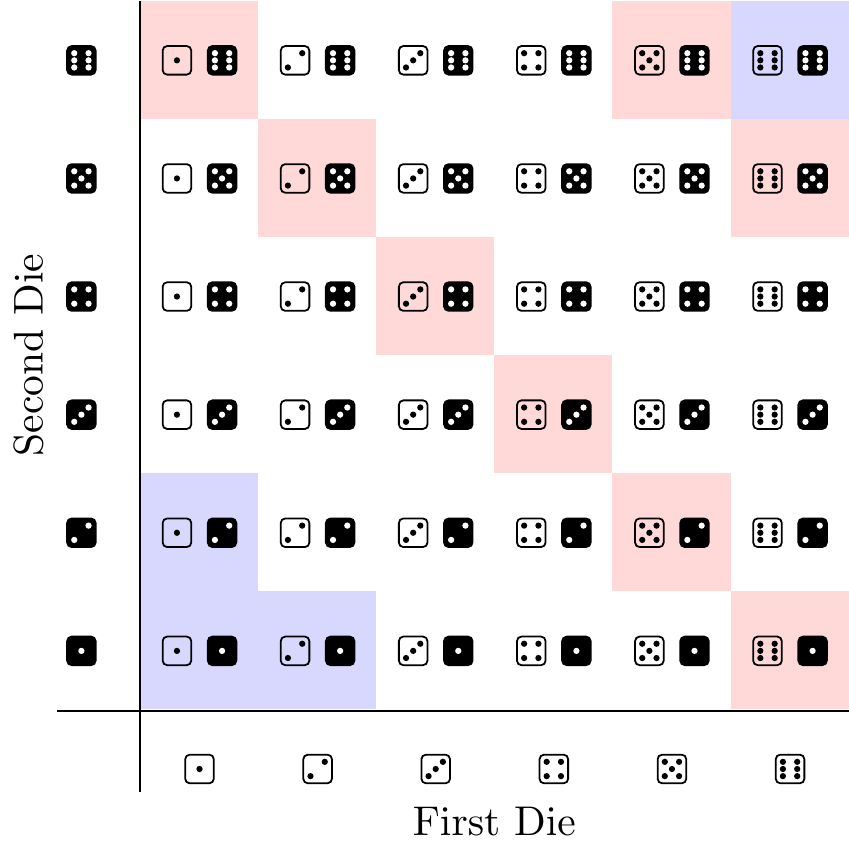
In order to win on the come-out roll, the shooter must roll a seven or eleven. This event is composed of the \(8\) outcomes highlighted in red in Figure 1.9. Therefore, the classical definition of probability (Definition 1.3) tells us that
\[ P(\text{win on come-out roll}) = P(\textcolor{red}{\text{roll seven or eleven}}) = \frac{\textcolor{red}{8}}{36} \approx 0.2222. \]
In order to lose on the come-out roll, the shooter must roll a two, three, or twelve (this scenario is called “craps,” lending the game its name). This event is composed of the \(4\) outcomes that are highlighted in blue in Figure 1.9. Therefore, Definition 1.3 tells us that
\[ P(\text{lose on come-out roll}) = P(\textcolor{blue}{\text{roll two, three, or twelve}}) = \frac{\textcolor{blue}{4}}{36} \approx 0.1111. \]
Note that winning and losing are not the only possible results of the come-out roll! If any other number is rolled, then that number becomes the point, and the round continues. We will analyze a complete round of craps later, in Example 7.1.
Following the reasoning from Example 1.9, it is easy to identify and correct Leibniz’s mistake in Example 1.2.
Solution 1.1 (Solving Leibniz’s problem). If we throw two fair dice, is it more likely that we roll an eleven or a twelve?
Examining the sample space Figure 1.9 from the craps example (Example 1.9), Leibniz’s mistake is easy to spot. Although it is true that rolling an eleven requires rolling one five and one six, there are two outcomes that correspond to doing so:

In contrast, there is only one outcome that corresponds to rolling a twelve:
Because the event of rolling an eleven contains twice as many outcomes as that of rolling a twelve, the classical definition of probability (Definition 1.3) implies that rolling an eleven is twice as likely.
In a nutshell, Leibniz’s mistake was that he applied Definition 1.3 to outcomes that were not equally likely. He treated eleven and twelve each as single outcomes, when the two outcomes are not equally likely.
It turns out that d’Alembert made essentially the same mistake in Example 1.3.
Our final example is another historical puzzle that stumped mathematicians for over a century. Although the solution only requires tools that we already have, it is far from obvious.
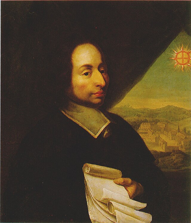
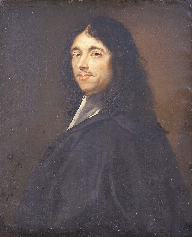
A satisfactory solution to the problem of points would not appear until over a century later. In a series of letters to one another, the French mathematicians Blaise Pascal and Pierre de Fermat devised the correct principle for dividing up the pot: each player should be awarded a fraction equal to their probability of winning the game. In fact, it was in the course of calculating this probability that Pascal invented “Pascal’s triangle,” the discovery for which he is perhaps best known today. We discuss Pascal’s triangle later in Proposition 2.6.
1.4 Exercises
Exercise 1.1 When outcomes are equally likely, we define the odds of the event \(A\) to be
\[ \text{odds}(A) \overset{\text{def}}{=}\frac{\text{number of outcomes in $A$}}{\text{number of outcomes not in $A$}}. \]
Odds are another way of describing chance that have their own advantages and disadvantages.
- Establish the following formulas for converting between probability and odds: \[ \begin{align} \text{odds}(A) &= \frac{P(A)}{1 - P(A)} & & \text{and} & P(A) &= \frac{\text{odds}(A)}{1 + \text{odds}(A)}. \end{align} \]
- In Example 1.4, what are the odds of winning a bet on red in roulette?
- In Example 1.6, what are the odds of not having an albino child?
Exercise 1.2 (Albinism revisited) Recall how albinism is inherited in Example 1.6. If an albino father (\(aa\)) and a carrier mother (\(Aa\)) have a child, what is the probability that their child is albino?
Exercise 1.3 (Secret Santa revisited) Suppose three friends participate in a Secret Santa gift exchange (Example 1.7).
- What is the probability that no one draws their own name?
- What is the probability that everyone draws their own name?
- What is the probability that exactly one person draws their own name?
Exercise 1.4 (Problem of points revisited) Consider Example 1.10, where two players are playing to 6 points, but now suppose the game is interrupted when the score is 4 to 3. What is the fair way to divide up the $100?
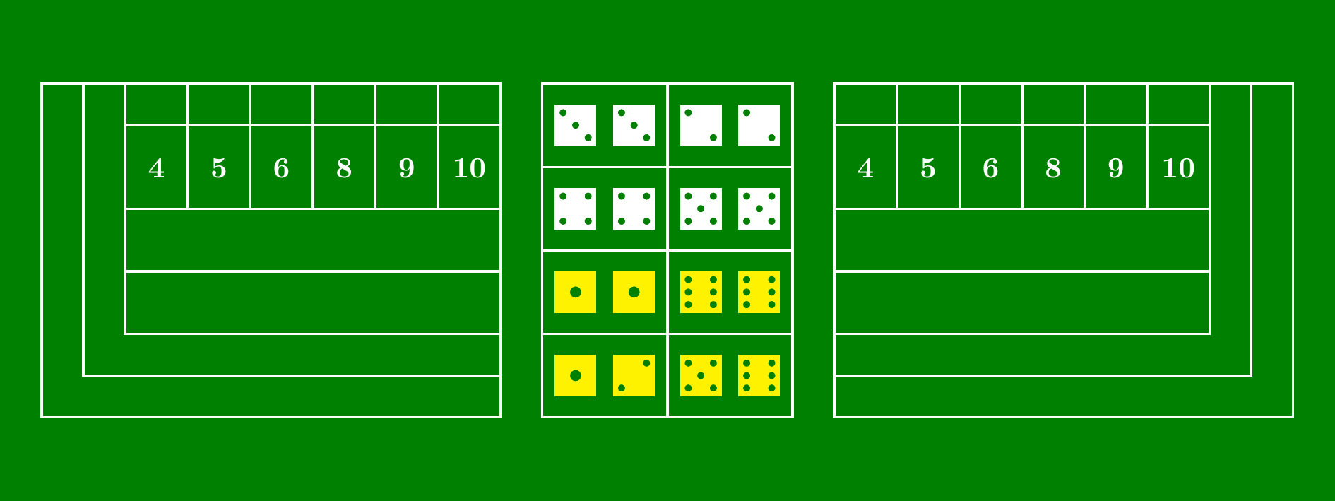
Exercise 1.5 (Efron’s dice) Our colleague Brad Efron invented a set of four six-sided dice (Gardner 1970), which are numbered differently from a traditional die:
- The faces on A are 4, 4, 4, 4, 0, 0.
- The faces on B are 3, 3, 3, 3, 3, 3.
- The faces on C are 6, 6, 2, 2, 2, 2.
- The faces on D are 5, 5, 5, 1, 1, 1.
One die is said to beat another if the number showing on that die is higher. For example, if A shows 4 and C shows 2, then A beats C.
- Calculate \(P(\text{A beats B})\), \(P(\text{B beats C})\), \(P(\text{C beats D})\), and \(P(\text{D beats A})\). What is strange about the probabilities you just calculated?
- (This is a true story.) Warren Buffett once challenged Bill Gates to a dice game with the four dice above. Each person would choose one of the dice and roll it, and the person with the higher number would win. After studying the dice, Gates said, “Okay, but you choose first.” Why did he say this?
Exercise 1.6 (Probability of the same color) You take out the four aces from a standard deck of playing cards (see Figure 1.6), as shown below.
Suppose you pick two of these cards at random. Your friend argues, “the colors are either the same or different, and there are the same number of cards of each color. So the probability that they are different and the probability that they are the same must both be \(\frac{1}{2}\)”. Do you agree?
(This exercise was adapted from a puzzle in Stewart (2010).)
Exercise 1.7 (Long run return) Recall the problem of points (Example 1.10). We will imagine having Players A and B repeatedly finish the game from the state they were interrupted in.
Using the frequentist interpretation of probability, explain why in the long run Player A will walk away with an average of $87.50 per round of the repeated game.
More generally, suppose you play a game you win with probability \(p\). When you win, you receive \(D\) dollars. Using the frequentist interpretation of probability, argue that if you play this game repeatedly, you will earn an average of \(pD\) dollars per round.