\[
\def\E{\text{E}}
\def\Var{\text{Var}}
\def\SD{\text{SD}}
\def\mean{\textcolor{red}{1.2}}
\]
In this chapter, we discuss how to calculate the expected value of a function of a random variable, \(\E[g(X)]\), and apply this to calculate the variance of a random variable. The discussion parallels Chapter 11 for discrete random variables.
Law of the Unconscious Statistician
In Example 20.1, we derived the PDF of \[ Y = g(X) = X^2, \] the area of a random square whose side length \(X\) is equally likely to be any number between \(0\) and \(1\).
To calculate \(\E[Y] = \E[X^2]\), we could use the PDF of \(Y\) we derived in Example 20.1. But deriving the PDF was a lot of work! Is there a way to calculate \(\E[g(X)]\) using just the PDF of \(X\)?
Fortunately, there is LotUS for continuous random variables, just as there was LotUS for discrete random variables (Chapter 11).
Theorem 21.1 (Law of the Unconscious Statistician) Let \(X\) be a continuous random variable with PDF \(f_X(x)\). Then, for any function \(g\), \[ \E[g(X)] = \int_{-\infty}^\infty g(x) f_X(x)\,dx. \tag{21.1}\]
Note that this is the same as discrete LotUS, with the PMF replaced by the PDF and the sum replaced by an integral.
Although Equation 21.1 is the obvious analog of discrete LotUS, it is not trivial to prove. We prove only a special case below.
We will prove Equation 21.1 under the assumption that \(g(x) \geq 0\) for all \(x\). This justifies LotUS for expectations like \(\E[X^2]\).
Let \(Y = g(X)\). Since \(Y\) is a non-negative random variable, we can apply Proposition 19.1 to calculate \(\E[Y]\).
\[\begin{align*}
\E[g(X)] = \E[Y] &= \int_0^\infty P(Y > t)\,dt \\
&= \int_0^\infty P(g(X) > t)\,dt \\
&= \int_0^\infty \int_{\textcolor{red}{x: g(x) > t}} f_X(x)\,d\textcolor{red}{x}\,dt \\
&= \int_{-\infty}^\infty \int_{\textcolor{blue}{0}}^{\textcolor{blue}{g(x)}} f_X(x)\,d\textcolor{blue}{t}\,dx & \text{(Fubini's theorem)} \\
&= \int_{-\infty}^\infty g(x) f_X(x)\,dx.
\end{align*}\]
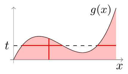
Notice that we used Fubini’s theorem to switch the order of integration from \(dx\,dt\) to \(dt\,dx\), turning a difficult integral into a trivial one. The intuition is quite simple and is illustrated below. The region of integration is the area between \(g(x)\) and the \(x\)-axis, shaded in orange below. This double integral can be evaluated in two ways: using horizontal slices, which requires integrating over the complicated set \(\{ x: g(x) > t \}\) for each \(t\), or using vertical slices, which is more straightforward.
Let’s use Theorem 21.1 to calculate the expected area.
Example 21.1 Using LotUS (Theorem 21.1), the expected area is \[
\begin{aligned}
\E[X^2] &= \int_{-\infty}^\infty x^2 f_X(x)\,dx \\
&= \int_0^1 x^2\cdot 1 \,dx \\
&= \frac{1}{3}.
\end{aligned}
\]
In this case, we know the PDF of
\(Y = X^2\) from
Example 20.1, so we can check our answer.
\[\begin{aligned}
\E[Y] &= \int_{-\infty}^\infty y f_Y(y)\,dy \\
&= \int_0^1 y \cdot \frac{1}{2\sqrt{y}} \,dy \\
&= \frac{1}{2} \int_0^1 \sqrt{y} \,dy \\
&= \frac{1}{3}.
\end{aligned}\]
We get the same answer this way as using LotUS, but LotUS is much simpler because it does not require first determining the PDF of the transformed random variable \(Y\).
Note that \(\E[g(X)]\) is not the same as \(g(\E[X])\). The expected value of a transformation is not the same as the transformation of the expected value.
In Example 21.1, the expected area \(\E[g(X)]\) is \(\frac{1}{3}\), but the area of a square with the expected side length is \[ g(\E[X]) = \E[X]^2 = \frac{1}{4}. \] In general, knowing the value of \(\E[X]\) is no help in computing \(\E[g(X)]\); when in doubt, use LotUS.
Variance
Now, we can define the variance of a continuous random variable, which is exactly the same as the variance of a discrete random variable.
Definition 21.1 (Variance) The variance of a random variable \(X\) is defined as \[ \Var[X] = \E[(X - \E[X])^2]. \] It measures the “typical” squared deviation from the “center” of the distribution (as measured by the expected value).
Since the quantity inside the expectation is a function of \(X\), it can be computed using LotUS (Theorem 21.1): \[ \E[(X - \E[X])^2] = \int_{-\infty}^\infty (x - \E[X])^2 f_X(x)\,dx. \tag{21.2}\]
Let’s calculate the variance of a random variable.
Example 21.2 (Variance of the Temperature in Iqaluit) In Example 18.5, we modeled the daily high temperature in Iqaluit, \(C\), as a continuous random variable with PDF \[ f_C(x) = \frac{1}{k} e^{-x^2/18}; -\infty < x < \infty. \]
How variable is the temperature in Iqaluit? We can measure this using \(\Var[C]\). To calculate \(\Var[C]\) according to Definition 21.1, we first must determine the expected value \(\E[C]\). Intuitively, the PDF Equation 18.7 is symmetric around zero (see Figure 18.7), so the center of mass must be zero. Let’s check that the \(\E[C]\) is indeed \(0\):
\[
\begin{aligned}
\E[C] &= \int_{-\infty}^\infty x \cdot \frac{1}{k} e^{-x^2/18}\,dx \\
&= -\frac{9}{k} e^{-x^2 / 18}\Big|_{-\infty}^\infty \\
&= 0.
\end{aligned}
\]
Now, the variance must be: \[
\begin{aligned}
\Var[C] &= \int_{-\infty}^\infty \underbrace{(x - 0)^2}_{x^2} \cdot \frac{1}{k} e^{-x^2/18}\,dx. \\
\end{aligned}
\]
This integral can be evaluated using integration by parts (with \(u = \frac{x}{k}\) and \(dv = xe^{-x^2 / 18}\)).
\[
\begin{aligned}
\int_{-\infty}^\infty x^2 \cdot \frac{1}{k} e^{-x^2/18}\,dx &= \overbrace{\frac{x}{k}}^u \cdot \overbrace{-9 e^{-x^2 / 18}}^v \Big|_{-\infty}^\infty - \int_{-\infty}^\infty \overbrace{-9e^{-x^2 / 18}}^v \overbrace{\frac{1}{k}\,dx}^{du} \\
&= 0 + 9 \underbrace{\int_{-\infty}^\infty \frac{1}{k} e^{-x^2 / 18}\,dx}_{= 1} \\
&= 9.
\end{aligned}
\]
In the last step, we used the fact that the integrand is a PDF.
So the variability of the daily high temperature in Iqaluit, as summarized by the variance, is \(9\).
What are the units of this variance? Because \(C\) is measured in Celsius, and we calculated \(\E[C^2]\), the units must be “degrees Celsius squared”. Because it’s hard to make sense of a square degree Celsius, we take the square root of the variance to obtain a measure of variability on the same scale as the original random variable.
Definition 21.2 (Standard Deviation) The standard deviation of a random variable \(X\) is defined as \[ \SD[X] = \sqrt{\Var[X]}, \] and its units are the same as \(X\).
Example 21.3 (Standard Deviation of the Temperature in Iqaluit) The standard deviation of the daily high temperature in Iqaluit is \[ \SD[C] = \sqrt{\Var[C]} = \sqrt{9} = 3^\circ \text{Celsius}. \] Looking at the PDF in Figure 18.7, this makes sense. The bulk of the probability is within \(\pm 3^\circ\) of the center (\(0^\circ\)).
In many situations, the variance is usually more easily computed using the “shortcut formula”.
Proposition 21.1 (Shortcut Formula for Variance) \[ \Var[X] = \E[X^2] - \E[X]^2 \]
Let \(\mu = \E[X]\). By Equation 21.2, the variance is \[
\begin{aligned}
\Var[X] &= \E[(X - \mu)^2] \\
&= \int_{-\infty}^\infty (x - \mu)^2 f_X(x)\,dx \\
&= \int_{-\infty}^\infty (x^2 - 2x\mu + \mu^2) f_X(x)\,dx & \text{(expand the square)} \\
&= \int_{-\infty}^\infty x^2 f_X(x)\,dx - \int_{-\infty}^\infty 2x\mu f_X(x)\,dx + \int_{-\infty}^\infty \mu^2 f_X(x)\,dx & \text{(split up terms)} \\
&= \underbrace{\int_{-\infty}^\infty x^2 f_X(x)\,dx}_{\E[X^2]} - 2\mu \underbrace{\int_{-\infty}^\infty x f_X(x)\,dx}_{\E[X] = \mu} + \mu^2 \underbrace{\int_{-\infty}^\infty f_X(x)\,dx}_{1} & \text{(pull out constants)} \\
&= \E[X^2] - 2\mu^2 + \mu^2 \\
&= \E[X^2] - \mu^2.
\end{aligned}
\]
Let’s apply this shortcut formula to measure the uncertainty in the time of the first click of a Geiger counter.
Example 21.4 Let \(T\) be the time of the first click of the Geiger counter from Example 18.7. How much uncertainty or variability is there in \(T\)?
First, we calculate \(\Var[T]\) using the shortcut formula \(\E[T^2] - \E[T]^2\). Note that we already determined in Example 19.2 that \(\E[T] = \frac{1}{\mean}\), so we just need to calculate \(\E[T^2]\). This requires LotUS and integration by parts. \[
\begin{aligned}
\E[T^2] &= \int_0^\infty x^2 \cdot \mean e^{-\mean x}\,dx \\
&= \underbrace{x^2}_u \cdot \underbrace{-e^{-\mean x}}_v \Big|_0^\infty - \int_0^\infty \underbrace{-e^{-\mean x}}_v \cdot \underbrace{2 x\,dx}_{du} \\
&= (0 - 0) + \frac{2}{\mean} \underbrace{\int_0^\infty x \cdot \mean e^{-\mean x}\,dx}_{\E[T] = \frac{1}{\mean}} \\
&= \frac{2}{\mean^2}
\end{aligned}
\]
Therefore, the variance is \[ \Var[T] = \E[T^2] - \E[T]^2 = \frac{2}{\mean^2} - \left(\frac{1}{\mean}\right)^2 = \frac{1}{\mean^2} \approx 0.694. \]
Note that this variance is in units of \(\text{minutes}^2\). To make this more interpretable, we take the square root to obtain the standard deviation:
\[ \SD[T] = \sqrt{\frac{1}{\mean^2}} \approx 0.833\ \text{minutes}. \]
Expectation and Variance of a Location-Scale Transformation
Any time we encounter an expectation of the form \(\E[g(X)]\), we should think “LotUS.” However, if the transformation is a location-scale transformation—that is, of the form \(g(x) = ax + b\) for constants \(a\) and \(b\)—we can bypass LotUS altogether.
Proposition 21.2 (Expectation of a Location-Scale Transformation) Let \(X\) be a random variable, and let \(a\) and \(b\) be constants. Then:
\[ \E[aX + b] = a\E[X] + b. \tag{21.3}\]
The easiest way to prove this is using LotUS (Theorem 21.1): \[
\begin{align}
\E[aX + b] &= \int_{-\infty}^\infty (ax + b) f_X(x)\,dx \\
&= a \underbrace{\int_{-\infty}^\infty x f_X(x)\,dx}_{\E[X]} + b \underbrace{\int_{-\infty}^\infty f_X(x)\,dx}_1 \\
&= a \E[X] + b.
\end{align}
\]
However, because we only proved LotUS for non-negative transformations \(g(x) \geq 0\), and \(ax + b\) is not guaranteed to be non-negative, we will provide an alternative proof using location-scale transformations.
Clearly, Equation 21.3 holds when \(a = 0\). When \(a \neq 0\), we showed in Proposition 20.3 that \(Y = aX + b\) has PDF \[ f_Y(y) = \frac{1}{|a|} f_X\Big(\frac{y - b}{a}\Big). \]
For simplicity, we will assume \(a > 0\) so that \(|a| = a\), but the proof for \(a < 0\) works similarly. \[
\begin{aligned}
\E[aX + b] &= \E[Y] \\
&= \int_{-\infty}^\infty y f_Y(y)\,dy \\
&= \int_{-\infty}^\infty y \frac{1}{a} f_X\Big(\frac{y - b}{a}\Big)\,dy \\
&= \int_{-\infty}^\infty (a x + b) f_X(x)\,dx & (y = ax + b) \\
&= a \underbrace{\int_{-\infty}^\infty x f_X(x)\,dx}_{\E[X]} + b \underbrace{\int_{-\infty}^\infty f_X(x)\,dx}_1 \\
&= a \E[X] + b
\end{aligned}
\]
There is also a simple formula for the variance of a location-scale transformation.
Proposition 21.3 (Variance of a Location-Scale Transformation) Let \(X\) be a random variable, and let \(a\) and \(b\) be constants. Then:
\[ \Var[aX + b] = a^2 \Var[X]. \tag{21.4}\]
This result is intuitive. Adding a constant \(b\) does not change the variability. Multiplying by a constant \(a\) scales the variability by a factor of \(a^2\) because variance is in squared units.
\[
\begin{aligned}
\Var[aX + b] &= \E[(aX + b - \E[aX + b])^2] & (\text{definition of variance}) \\
&= \E[((aX + b) - (a\E[X] + b))^2] & (\text{expectation of a location-scale transform}) \\
&= \E[(a(X - \E[X]) + \underbrace{(b - b)}_0)^2] & (\text{regroup terms}) \\
&= \E[a^2 (X - \E[X])^2] & (\text{factor out $a^2$}) \\
&= a^2 \E[(X - \E[X])^2] & (\text{expectation of a scale transform}) \\
&= a^2 \Var[X] & (\text{definition of variance})
\end{aligned}
\]
Using Proposition 21.2 and Proposition 21.3, it is easy to calculate the expectation and variance of the temperature in Fahrenheit, if we already know the expectation and variance in Celsius.
Example 21.5 (Expectation and Variance of the Temperature in Fahrenheit) In Example 21.2, we showed that the expected value and variance of the temperature in Celsius were \[
\begin{aligned}
\E[C] &= 0 & \text{and} & & \Var[C] &= 9.
\end{aligned}
\]
The temperature in Fahrenheit is a location-scale transformation, \[ F = \frac{9}{5} C + 32, \] where \(a = \frac{9}{5}\) and \(b = 32\). Therefore, by Proposition 21.2, the expected value is \[
\begin{aligned}
\E[F] &= \E\left[\frac{9}{5}C + 32\right] \\
&= \frac{9}{5} \E[C] + 32 \\
&= 32,
\end{aligned}
\] and by Proposition 21.3, the variance is \[
\begin{aligned}
\Var[F] &= \Var\Big[\frac{9}{5}C + 32\Big] \\
&= \left(\frac{9}{5}\right)^2 \Var[C] \\
&= 29.16.
\end{aligned}
\]