9 Expected Value

A random variable can take on many possible values. How do we reduce these values to a single number summary?

You may be know that one way to summarize a list of numbers is the average (or mean). For example, the list of six numbers \[ 1, 1, 2, 3, 3, 10 \tag{9.1}\] can be summarized by their average: \[ \bar x = \frac{1 + 1 + 2 + 3 + 3 + 10}{6} = \frac{20}{6} \approx 3.33. \tag{9.2}\]

There is another way to calculate this average. Instead of summing over the six numbers, we can sum over the four distinct values, $1$, $2$, $3$, and $10$, weighting each value by how often it occurs: \[ \bar x = \frac{2}{6} \cdot 1 + \frac{1}{6} \cdot 2 + \frac{2}{6} \cdot 3 + \frac{1}{6} \cdot 10 = \frac{20}{6} \approx 3.33. \tag{9.3}\]

Equation 9.3 is the idea behind the summary of a random variable that we discuss in this chapter, called the expected value.

9.1 Definition

Like Equation 9.3, the expected value sums over the possible values of the random variable, weighting each value by its probability.

Definition 9.1 (Expected value of a discrete r.v.) Let $X$ be a discrete random variable with PMF $f_X(x)$. Then, the expected value (or expectation or EV) of $X$ is \[ \text{E}\!\left[ X \right] \overset{\text{def}}{=}\sum_x x f_X(x) = \sum_x xP(X = x), \tag{9.4}\]

where the sum is taken over all possible values $x$.

We now illustrate Definition 9.1 with a simple example.

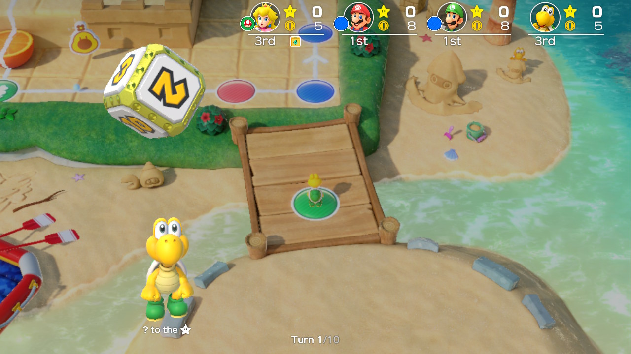
Example 9.1 (Expected value of Koopa’s die) The numbers in Equation 9.1 are in fact the six faces of the special die that Koopa can roll in the game Super Mario Party. In this game, players roll a die to determine how many spaces they move, as shown in Figure 9.1.

Figure 9.1: Koopa Troopa rolling his special die in Super Mario Party

If Koopa rolls his special die, then the number of spaces he moves is a random variable $X$ with PMF

$x$	$1$	$2$	$3$	$10$
$f_X(x)$	$\frac{2}{6}$	$\frac{1}{6}$	$\frac{2}{6}$	$\frac{1}{6}$

so the expected value is \[ \text{E}\!\left[ X \right] = \frac{2}{6} \cdot 1 + \frac{1}{6} \cdot 2 + \frac{2}{6} \cdot 3 + \frac{1}{6} \cdot 10 = \frac{20}{6} \approx 3.33. \]

Another option in Super Mario Party is to roll a standard die with faces labeled $1$ to $6$. If Koopa rolls a standard die, then the number of spaces he moves is a random variable $Y$ with PMF

$y$	$1$	$2$	$3$	$4$	$5$	$6$
$f_Y(y)$	$\frac{1}{6}$	$\frac{1}{6}$	$\frac{1}{6}$	$\frac{1}{6}$	$\frac{1}{6}$	$\frac{1}{6}$

so the expected value is \[ \text{E}\!\left[ Y \right] = \frac{1}{6} \cdot 1 + \frac{1}{6} \cdot 2 + \frac{1}{6} \cdot 3 + \frac{1}{6} \cdot 4 + \frac{1}{6} \cdot 5 + \frac{1}{6} \cdot 6 = 3.5, \] We see that Koopa is “expected” to move further with a standard die than his special die, which suggests that a standard die is “better.” We make this precise in the next section.

Notice that $3.33$ is not even a possible value of $X$, nor is $3.5$ a possible value of $Y$. In what sense then are these values “expected”? In the next section, we discuss various ways to interpret the expected value.

9.2 Interpretations

Just as the probability can be interpreted as the long-run frequency, the expected value can be interpreted as the long-run average when the experiment is repeated over and over. That is, if Koopa rolls his special die repeatedly, generating many values $X_1, X_2, X_3, \dots$, then \[ \lim_{n\to\infty} \frac{X_1 + X_2 + \dots + X_n}{n} = \frac{20}{6}.\] Similarly, if Koopa rolls a standard die repeatedly, generating many values $Y_1, Y_2, \dots$, then \[ \lim_{n\to\infty} \frac{Y_1 + Y_2 + \dots + Y_n}{n} = 3.5.\]

The code below simulates $n = 10000$ rolls of both dice and calculates a running average.

Notice that the average of the standard die settles around 3.5, while the average of the special die settles around a lower value, 3.33. This means that Koopa will be able to move, on average, more spaces per roll with a standard die than the special die, after many rolls.

However, this does not mean that the standard die is better than the special die in all situations. For example, if it is the last turn of the game and Koopa needs to move 8 spaces to win, then the special die is his only hope for victory; the long-run performance of the standard die is little consolation.

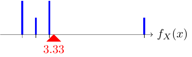
There is also a physical interpretation of expected value: it is where the PMF of the random variable “balances”. That is, the expected value is the center of mass of the PMF. For example, the PMF for Koopa’s special die is shown in Figure 9.2. If we imagine these probability masses on a scale, the scale will balance if the fulcrum is placed at the expected value $3.33$.

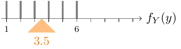
Figure 9.2: PMF and expected value of Koopa’s special die

Likewise, if we put the probability masses for a standard die on a scale, the scale will balance if the fulcrum is placed at the expected value $3.5$.

Figure 9.3: PMF and expected value of a standard die

To prove this, we need to quantify the rotational force (or torque) that each “weight” exerts about the fulcrum. If a weight $p$ (probability, in this case) is $d$ units to the left of the fulcrum, then the weight will tend to rotate the bar counterclockwise and the torque is $p\cdot d$. On the other hand, if the weight is $d$ units to the right of the fulcrum, then the weight will tend to rotate the bar clockwise and the torque is $-p\cdot d$. In order for the bar to balance, the total torque about the fulcrum from all weights must be $0$.

Proposition 9.1 (Expected value is the center of mass) Let $X$ be a random variable. Then, $\text{E}\!\left[ X \right]$ is the center of mass of the PMF of $X$.

Proof

If the fulcrum is placed at $\text{E}\!\left[ X \right]$, then the torque exerted by a “weight” $p = f_X(x)$ at $x$ would be \[ p \cdot d = f_X(x) \cdot (\text{E}\!\left[ X \right] - x). \] Hence, the total torque about the fulcrum is \[\begin{align*} \sum_x f_X(x) \cdot (\text{E}\!\left[ X \right] - x) &= \sum_x f_X(x) \cdot \text{E}\!\left[ X \right] - \sum_x f_X(x) \cdot x \\ &= \text{E}\!\left[ X \right] \underbrace{\sum_x f_X(x)}_1 - \text{E}\!\left[ X \right] \\ &= 0. \end{align*}\] Therefore, the total torque about the fulcrum is $0$, so the expected value is the center of mass.

9.3 Examples

In this section, we practice calculating and interpreting the expected values of different random variables.

Example 9.2 (Expected value of roulette bets) Recall Example 8.2, where we defined the random variables $\S$ and $\RR$, representing the profits from a $1 bet on the single number 23 and a $1 bet on red, respectively.

Although the bets are very different, their expected values are the same: \[\begin{align*} \text{E}\!\left[ \S \right] &= \frac{1}{38} \cdot 35 + \frac{37}{38} \cdot (-1) = -\frac{1}{19} \\ \text{E}\!\left[ \RR \right] &= \frac{18}{38} \cdot 1 + \frac{20}{38} \cdot (-1) = -\frac{1}{19}. \end{align*}\]

This means that if we were to repeatedly bet on 23 or repeatedly bet on red, then we would lose $\$1/19 \approx \$0.053$ per bet in the long run. Although their expected values are the same, the two bets are obviously very different. With a bet on 23, we hardly ever win, but when we do, the $35 profit makes up for all the bets we lose.

The code below simulates 10000 spins of a roulette wheel and calculates a running average of the profits from the two bets.

Notice that the average profit fluctuates much more with a bet on a single number than a bet on red, but they both settle around $-0.053$. (If the gray line is still fluctuating, try increasing the number of spins $n$.)

Another way to make sense of the expected value is to consider the “center of mass” interpretation. Although the PMFs of $\RR$ and $\S$ are very different, they happen to balance at the same fulcrum of $-1/19$.

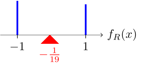
Figure 9.4: The random variables $S$ (blue) and $R$ (red) have very different PMFs but balance at the same expected value of $-1/19$.

In fact, all roulette bets have the same expected value of $-\frac{1}{19}$! Therefore, expected value is no help for deciding between these two bets. In Chapter 11, we will develop other summaries that distinguish these bets.

Expected values are also the basis for an important technique in medical diagnostics called pooled testing.

Example 9.3 (Pooled testing)

At the height of the COVID-19 pandemic, labs were analyzing thousands of COVID tests per day, which was both time-consuming and expensive. They used a strategy called pooled testing to make the process more efficient.

Suppose a lab has a batch of $10$ samples to test for COVID. They could run $10$ tests, one for each sample. But they could instead pool the samples into one large sample and test this pooled sample once. If this test comes back negative, then they can conclude that none of the $10$ samples had COVID, after only $1$ test! However, if this test comes back positive, then each of the $10$ samples has to be tested individually.

Figure 9.5: A lab technician processing samples from COVID tests.

Pooled testing is most effective when the positivity rate is low, since usually none of the samples in a batch will have COVID, so only $1$ test is needed for the entire batch.

To make this precise, we calculate the expected value of $T$, the number of tests under pooled testing. We will assume that the positivity rate is $p$ and that the samples are independent. There are two possibilities: either $T = 1$ (if none of the samples have COVID) or $T = 11$ (if at least one of the samples has COVID). The PMF of $T$ is:

$t$	$1$	$11$
$f_T(x)$	$(1 - p)^{10}$	$1 - (1 - p)^{10}$

The expected number of tests is therefore: \[ \text{E}\!\left[ T \right] = 1 \cdot (1 - p)^{10} + 11 \cdot (1 - (1 - p)^{10}) = 11 - 10(1 - p)^{10}. \tag{9.5}\] Since a lab will typically process many batches in a day, this expected value represents the average number of tests per batch with pooled testing.

When will pooled testing be more efficient than testing each sample individually? Precisely when Equation 9.5 is less than $10$, the number of tests per batch if each sample were tested individually: \[ \begin{align} \text{E}\!\left[ T \right] &< 10 \\ 11 - 10(1 - p)^{10} &< 10 \\ p &< 1 - 0.1^{1/10} \approx .206. \end{align} \] That is, as long as the positivity rate is lower than 20%, then pooled testing will be more efficient. Since positivity rates were typically under 10%, pooled testing was an effective strategy during the COVID-19 pandemic.

We conclude this section by illustrating a few ways to calculate the expectation of a random variable that follows a named distribution.

Example 9.4 (Expected number of albino children) In Example 8.8, we argued that if a couple who are carriers of albinism have 5 children, then the number of albino children $X$ is a $\textrm{Binomial}(n= 5, p= .25)$ random variable. We derived its PMF to be:

$x$	$0$	$1$	$2$	$3$	$4$	$5$
$f_X(x)$	$\frac{243}{1024}$	$\frac{405}{1024}$	$\frac{270}{1024}$	$\frac{90}{1024}$	$\frac{15}{1024}$	$\frac{1}{1024}$

What is $\text{E}\!\left[ X \right]$, the expected number of albino children that the couple has? We can calculate it directly from the probabilities in the table above:

\[ \begin{aligned} \text{E}\!\left[ X \right] &= 0 \cdot \frac{243}{1024} + 1 \cdot \frac{405}{1024} + 2 \cdot \frac{270}{1024} \\ &\qquad + 3\cdot \frac{90}{1024} + 4\cdot \frac{15}{1024} + 5\cdot \frac{1}{1024} \\ &= 1.25. \end{aligned} \]

Note that the expected value in Example 9.4 was simply the number of children ($n=5$) times the probability that each child is albino ($p=.25$). This is no accident; the expected value of a binomial random variable will always be $np$. We derive this useful formula next.

Example 9.5 (Binomial expectation) Let $X \sim \text{Binomial}(n,p)$. Using the combinatorial identity Proposition 2.5, we see that \[\begin{align*} \text{E}\!\left[ X \right] &= \sum_{k=0}^n k \binom{n}{k} p^k (1-p)^{n-k} & \text{(definition of expectation)} \\ &= \sum_{k=1}^n k \binom{n}{k} p^k (1-p)^{n-k} & \text{($i=0$ term is $0$)} \\ &= np \sum_{k=1}^n \binom{n-1}{k-1} p^{k-1} (1-p)^{n-k} & \text{(pull out $np$)} \\ &= np \sum_{j=0}^{n-1} \underbrace{\binom{n-1}{j} p^j (1-p)^{n-1-j}}_{\text{Binomial}(n-1, p)\ \text{PMF}} & \text{($j = k - 1$)} \\ &= np, \end{align*}\] where the last step follows because every PMF must sum to $1$.

Therefore, whenever we encounter a $\text{Binomial}(n, p)$ random variable, we know its expectation will be $np$, so we do not need to calculate it from Definition 9.1, as we did in Example 9.4.

Note that since a $\text{Bernoulli}(p)$ random variable is simply a binomial random variable where $n=1$, Example 9.5 also implies that the expected value of a Bernoulli random variable is $p$.

The derivation in Example 9.5 was quite cumbersome. In Example 14.3, we will present an alternative derivation of the binomial expectation that involves less algebra and offers more intuition about why the expected value is $np$.

9.4 Paradoxes

Expected value can yield surprising answers, especially when infinities are involved. This section presents two fascinating historical examples.

Example 9.6 (Pascal’s wager) Should we believe in God? Suppose $p$ is the probability that God exists.

If we were to adopt the belief that God exists and live a lifestyle accordingly, we incur a finite amount of loss, associated with sacrificing certain pleasures and luxuries.

After dying, if God does exist, we would enjoy infinite time in heaven, which would equate to infinite gains. If God does not exist, then there is nothing after.

On the other hand, if we did not believe in God and God turned out to be real, we would suffer infinite losses in hell.

The quasi-EV calculation, if we were to believe in God, would be \[ \text{E}\!\left[ X \right] = -\text{finite sacrifices} + p \cdot \text{infinite gains} + (1-p) \cdot 0 > \infty \] as long as $p > 0$, if $X$ represents our lifetime gains. Pascal argued that since no one can ever be certain of God’s existence, $p \neq 0$, and so, we should all strive to believe in God.

Example 9.7 (St. Petersburg paradox) You are offered the following bet based on tosses of a fair coin. A pot initially contains $2. Each time the coin lands tails, the amount in the pot is doubled. The game ends when the coin lands heads, at which point you win whatever is in the pot. For example,

If the coin lands heads on the first toss, you win $2.
If the coin lands heads on the fourth toss (TTTH), you win $16, since the pot was doubled three times before the heads appeared.

Clearly, you should be willing to pay at least $2 to play this game, since you always win at least $2. Before reading the solution, think about how much you would be willing to pay.

The expected value is sometimes considered a fair price to pay. Let $X$ represent the payout. Then the PMF of $X$ is

$x$	$2$	$4$	$8$	$16$	$32$	$\dots$
$f_X(x)$	$\frac{1}{2}$	$\frac{1}{4}$	$\frac{1}{8}$	$\frac{1}{16}$	$\frac{1}{32}$	$\dots$

The expected value is therefore \[\begin{align*} \text{E}\!\left[ X \right] &= \underbrace{2 \cdot \frac{1}{2}}_{1} + \underbrace{4 \cdot \frac{1}{4}}_{1} + \underbrace{8 \cdot \frac{1}{8}}_{1} + \underbrace{16 \cdot \frac{1}{16}}_{1} + \cdots \\ &= \infty. \end{align*}\] This implies that you should be willing to pay any price to enter this game since the expected profit is infinite! This is a paradox because few people would be willing to pay more than $100 to play such a game.

This paradox was made famous by Daniel Bernoulli in 1738, who proposed one resolution that we will examine in Example 11.2.

9.5 Tail Sum Formula

In Section 8.5, we introduced the geometric distribution. What is the expected value of a geometric random variable? We could attempt to evaluate the sum \[ \text{E}\!\left[ N \right] = \sum_{n=1}^\infty n \cdot (1 - p)^{n-1} p, \] but this is not an easy sum to evaluate. The optional section below explains how.

Evaluating the sum for geometric expectation

First, we factor out $p$: \[\text{E}\!\left[ N \right] = p \sum_{n=1}^\infty n (1 - p)^{n-1}.\]

To evaluate the summation, we first define $x = 1 - p$ to obtain \[ \sum_{n=1}^\infty n(1 - p)^{n-1} = \sum_{n=1}^\infty n x^{n-1}. \]

Notice that each term is the derivative of $x^n$. In other words, this is the term-by-term derivative of a power series:

\[ \sum_{n=1}^\infty n x^{n-1} = \sum_{n=1}^\infty \frac{d}{dx} x^{k} = \frac{d}{dx} \sum_{n=1}^\infty x^{n} = \frac{d}{dx} \frac{x}{1 - x}. \]

In the last line above, we used the fact that the sum was a geometric series and $|x| = |1 - p| < 1$. Taking the derivative with respect to $x$, we obtain:

\[ \sum_{n=1}^\infty n(1 - p)^{n-1} = \frac{(1 - x) + x}{(1 - x)^2} = \frac{1}{p^2}. \]

Multiplying by $p$, we obtain the expected value \[ \text{E}\!\left[ N \right] = p \sum_{n=1}^\infty n(1 - p)^{n-1} = p \frac{1}{p^2} = \frac{1}{p}. \]

Instead, we will calculate this expected value by using an alternative formula, derived in the result below.

Proposition 9.2 (Tail sum formula for expectation) Let $X$ be a random variable that is nonnegative-integer-valued. That is, it takes on the values $0, 1, 2, ...$. Then

\[ \text{E}\!\left[ X \right] = \sum_{x=0}^\infty P(X > x) = \sum_{x=0}^\infty (1 - F(x)). \tag{9.6}\]

Proof 1: Visual Proof

Because $X$ is nonnegative-integer-valued, the expected value is \[ \text{E}\!\left[ X \right] = \sum_{x=0}^\infty x \cdot P(X = x). \] Another way to interpret each term in this summation, $x \cdot P(X = x)$, is \[ \underbrace{P(X = x) + P(X = x) + \dots + P(X = x)}_{\text{$x$ times}}. \]

Therefore, we can organize the calculation of $\text{E}\!\left[ X \right]$ in a triangular array as follows: \[ \begin{array}{l|ccccccccc} \phantom{+} 1 \cdot P(X = 1) & & P(X = 1) \\ + 2\cdot P(X = 2) & + & P(X = 2) & + & P(X = 2) \\ + 3\cdot P(X = 3) & + & P(X = 3) & + & P(X = 3) & + & P(X = 3) \\ + \qquad \vdots & + & \vdots & + & \vdots & + & \vdots & + & \ddots \\ \hline \qquad \text{E}\!\left[ X \right] & & P(X > 0) & + & P(X > 1) & + & P(X > 2) & + & \dots. \end{array} \]

The definition of expected value says to first sum each row of the triangular array to obtain terms of the form $x \cdot P(X = x)$, then sum these terms to obtain the expected value. But the entries of the array can be summed in any order (because they are non-negative). If we instead first sum each column of the array, then we obtain terms of the form $P(X > x)$, which we can sum to obtain the expected value.

Proof 2: Algebraic Proof

We can also write this proof using summations. \[\begin{align*} \sum_{x=0}^\infty P(X > x) &= \sum_{x=0}^\infty \sum_{k=x+1}^\infty P(X = k) \\ &= \sum_{k=1}^\infty \sum_{x = 1}^k P(X = k) \\ &= \sum_{k=1}^\infty k \cdot P(X = k) \\ &= \text{E}\!\left[ X \right]. \end{align*}\]

The key trick was switching the order of the two summations in the second line. This is equivalent to switching from summing over columns to summing over rows in the visual proof above.

Proposition 9.2 provides an easier way to calculate the expected value of a $\text{Geometric}(p)$ random variable.

Example 9.8 (Geometric expectation by the tail sum formula) Let $N$ be a $\text{Geometric}(p)$ random variable. Since $N$ only takes on the values 1, 2, 3, …, we can apply Proposition 9.2. But we first need to determine $P(N > x)$.

We can calculate $P(N > x)$ by summing the geometric PMF, or by observing that $\{ N > x\} = \{ \text{first $x$ tosses were tails} \}$, so \[ P(N > x) = (1 - p)^x; \qquad x=0, 1, 2, \dots. \]

Now we can apply Proposition 9.2.

\[ \begin{aligned} \text{E}\!\left[ N \right] &= \sum_{x=0}^\infty P(N > x) \\ &= \sum_{x=0}^\infty (1 - p)^x \\ &= \frac{1}{1 - (1 - p)} & \text{(sum of geometric series)} \\ &= \frac{1}{p}. \end{aligned} \]

In Example 16.4, we will see an even slicker way to derive this expected value using conditional expectations.

Armed with Example 9.8, we can make quick work of problems like the following.

Example 9.9 (Expected number of rolls in craps) In Example 8.10, we showed that if the point is $5$, then the number of (additional) rolls until the round ends is a $\text{Geometric}(p=\frac{10}{36})$ random variable $X$. The expected number of additional rolls is therefore \[ \text{E}\!\left[ X \right] = \frac{1}{p} = \frac{1}{\frac{10}{36}} = 3.6. \]

9.6 Exercises

Exercise 9.1 (Expected number of Secret Santa matches) In Exercise 8.2, you derived the PMF of $X$, the number of friends in a Secret Santa gift exchange who draw their own name. Now, calculate and interpret $\text{E}\!\left[ X \right]$, the expected number of friends who draw their own name.

Exercise 9.2 (Expected points in a one-and-one) In Exercise 8.1, you derived the PMF of $X$, the number of points in a one-and-one. What is the expected number of points in a one-and-one, assuming $p = 0.75$?

Exercise 9.3 (EV of a field bet in craps) In Exercise 8.3, you derived the PMF of the profit from a $1 field bet in craps. Use this to calculate the expected profit. How does this bet compare to the pass-line bet (Example 7.1)?

Exercise 9.4 (Making the field bet fair) Continuing Exercise 9.3, what would the payout have to be for 2 and 12 have to be, instead of 2-to-1, in order for the field bet to be fair? Here, fair means expected net winnings is 0.

Exercise 9.5 (Another pooled testing strategy) In Example 9.3, we discussed one pooled testing strategy for COVID-19 and determined when it was more efficient than testing each sample individually. Now consider the following strategy for testing a batch of 10 samples:

Pool 5 samples into one medium sample, and pool the other 5 samples into another medium sample.
Pool these two medium samples into one large sample.
Test the large sample.
- If the test comes back negative, then none of the 10 samples have COVID.
- If the test comes back positive, then test each of the medium samples.
  - If the test comes back negative, then none of the 5 samples have COVID.
  - If the test comes back positive, then test each sample individually.

Calculate the expected number of tests with this strategy in terms of $p$, the positivity rate. When is this strategy more efficient than testing each sample individually? Compare with the results from Example 9.3.

Exercise 9.6 (Expectations in roulette) Continuing Exercise 8.6, calculate

$\text{E}\!\left[ X \right]$
$\text{E}\!\left[ W \right]$

Exercise 9.7 (Expected number of keys to try) Continuing Exercise 9.7, calculate

$\text{E}\!\left[ X \right]$ (Hint: You may find the identity from Exercise 2.22 helpful. However, is should also be obvious from Proposition 9.1 what the EV is.)
$\text{E}\!\left[ Y \right]$

Which strategy appears to be better?