28 The Law of Large Numbers and Interpreting Probability

In Chapter 1, we discussed the frequentist interpretation of probability, which says that the probability $P(A)$ corresponds to the long-run frequency of the event $A$ in repeated trials. In Chapter 9, we discussed how the expected value $\text{E}\!\left[ X \right]$ corresponds to the long-run average of repeated realizations of the random variable $X$. In this chapter, we will develop a mathematical framework in which these assertions can be proven. The resulting theorem is called the Law of Large Numbers.

Here is the mathematical framework: repeated realizations of a random variable $X$ can be modeled as independent and identically distributed (i.i.d.) random variables $X_1, X_2, X_3, \dots$, all with the same distribution as $X$.

The average of the first $n$ observations is called the sample mean, which we write as follows: \[ \bar{X}_n \overset{\text{def}}{=}\frac{X_1 + X_2 + \dots + X_n}{n}. \] We will show that, under the assumption that $\mu \overset{\text{def}}{=}\text{E}\!\left[ X_i \right]$ and $\sigma^2 \overset{\text{def}}{=}\text{Var}\!\left[ X_i \right]$ exist and are finite, \[ \bar{X}_n \text{ ``$\to$'' } \mu \qquad \text{as $n\to\infty$}. \tag{28.1}\] We put quotes around the convergence arrow because this is different from the limits you encountered in calculus; the left-hand side is a random variable, while the right-hand side is a constant. We will also need to define what is meant by “convergence” in this context.

An informal way to justify Equation 28.1 is to calculate the expectation and variance of $\bar{X}_n$.

Proposition 28.1 (Expectation and variance of $\bar{X}_n$) Let $X_1, \dots, X_n$ be i.i.d. with $\mu\overset{\text{def}}{=}\text{E}\!\left[ X_i \right]$ and $\sigma^2 \overset{\text{def}}{=}\text{Var}\!\left[ X_i \right]$. Then,

\[ \begin{align} \text{E}\!\left[ \bar{X}_n \right] &= \mu & \text{Var}\!\left[ \bar{X}_n \right] &= \frac{\sigma^2}{n}. \end{align} \]

Proof

First, by linearity of expectation (Theorem 14.2), \[ \begin{align} \text{E}\!\left[ \bar{X}_n \right] &= \text{E}\!\left[ \frac{\sum_{i=1}^n X_i}{n} \right] \\ &= \frac{1}{n} \sum_{i=1}^n \text{E}\!\left[ X_i \right] \\ &= \frac{1}{n} \sum_{i=1}^n \mu \\ &= \frac{1}{n} n\mu \\ &= \mu. \end{align} \]

For the variance, we use properties of covariance (Proposition 15.1), as well as the fact that $X_i$ and $X_j$ are independent for $i \neq j$ (so $\text{Cov}\!\left[ X_i, X_j \right] = 0$). \[\begin{align*} \text{Var}\!\left[ \bar{X}_n \right] &= \text{Cov}\!\left[ \frac{1}{n} \sum_{i=1}^n X_i, \frac{1}{n} \sum_{i=1}^n X_i \right] \\ &= \frac{1}{n^2} \sum_{i=1}^n \sum_{j=1}^n \text{Cov}\!\left[ X_i, X_j \right] \\ &= \frac{1}{n^2} \sum_{i=1}^n \text{Cov}\!\left[ X_i, X_i \right] \\ &= \frac{1}{n^2} \sum_{i=1}^n \text{Var}\!\left[ X_i \right] \\ &= \frac{1}{n^2} \sum_{i=1}^n \sigma^2 \\ &= \frac{1}{n^2} \cdot n \sigma^2 \\ &= \frac{\sigma^2}{n}. \end{align*}\]

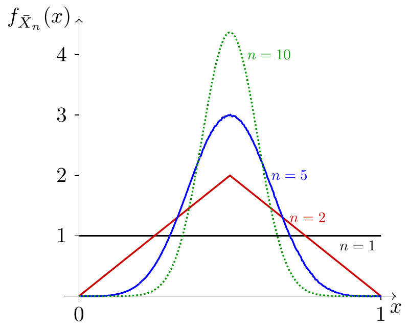
As $n$ increases, the expected value remains constant at $\mu$, while the variance decreases to zero. This means that the probability will become more and more “concentrated” near $\mu$ as $n$ increases. Figure 28.1 shows what happens for i.i.d. $\textrm{Uniform}(a= 0, b= 1)$ random variables $X_1, X_2, X_3, \dots$.

Figure 28.1: PDF of $\bar X_n$ for $n=1, 2, 5, 10$, where $X_1, X_2, \dots$ are i.i.d. $\textrm{Uniform}(a= 0, b= 1)$.

We can also explore this phenomenon by simulation. The simulation below simulates $\bar{X}_n$ for i.i.d. $\textrm{Exponential}(\lambda=1)$ random variables.

Try increasing $n$, and observe how $\bar{X}_n$ “concentrates” around the expected value $\mu = 1$ as $n$ increases.
Try changing the distribution (Poisson? normal?), and verifying that $\bar{X}_n$ behaves in the same way.

28.1 Convergence in Probability

The simulation above illustrates how the random variable $\bar{X}_n$ “concentrates” around $\mu$ as $n$ increases. To make this precise, we need the following definition.

Definition 28.1 (Convergence in probability) A sequence of random variables $Y_1, Y_2, Y_3, \dots$ is said to converge in probability to a constant $c$ if for any $\varepsilon > 0$, \[ \lim_{n\to\infty} P(|Y_n - c| > \varepsilon) = 0. \tag{28.2}\]

We write $Y_n \overset{p}{\to} c$.

That is, no matter how small $\varepsilon$ is, $Y_n$ will eventually be within $\varepsilon$ of $c$ with probability close to $1$.

The Law of Large Numbers, which we prove in Theorem 28.2, is simply the statement that \[ \bar{X}_n \overset{p}{\to} \mu. \]

Clearly, convergence in probability requires that we be able to provide bounds on how far random variables can deviate from their expected value. In other words, these bounds indicate how much random variables “concentrate” around their expected value. For this reason, they are called concentration inequalities.

28.2 Concentration Inequalties

Theorem 28.1 (Markov’s inequality) If $X$ is a nonnegative random variable, then \[ P(X \geq a) \leq \frac{\text{E}\!\left[ X \right]}{a} \tag{28.3}\] for any $a > 0$.

Proof

For $a > 0$, let \[ I_{\{ X \geq a\}} = \begin{cases} 1, & X \geq a \\ 0, & X < a \end{cases}. \] In other words, $I_{\{ X \geq a\}}$ is the indicator of whether $X \geq a$ or not. Then, $a I_{\{ X \geq a\}} \leq X$, and so, \[ \text{E}\!\left[ a I_{\{ X \geq a\}} \right] \leq \text{E}\!\left[ X \right]. \] The left-hand side becomes $a \text{E}\!\left[ I_{\{ X \geq a\}} \right] = a P(X \geq a)$. Finally, we divide both sides by $a$ to obtain the desired result.

The next result, Chebyshev’s inequality, is a corollary of Markov’s inequality.

Corollary 28.1 (Chebyshev’s inequality) Let $Y$ be a random variable with $\mu\overset{\text{def}}{=}\text{E}\!\left[ Y \right]$ and $\sigma^2 \overset{\text{def}}{=}\text{Var}\!\left[ Y \right]$ finite. Then: \[ P(\lvert Y - \text{E}\!\left[ Y \right] \rvert \geq a) \leq \frac{\text{Var}\!\left[ Y \right]}{a^2} \tag{28.4}\] for any $a > 0$.

Proof

First, we square both sides inside the probability on the left-hand side of Equation 28.4: \[ P(\lvert Y - \text{E}\!\left[ Y \right] \rvert \geq a) = P((Y - \text{E}\!\left[ Y \right])^2 \geq a^2). \] Now, since $(Y - \text{E}\!\left[ Y \right])^2$ is a nonnegative random variable, we can use Theorem 28.1 to obtain \[ P( (Y - \text{E}\!\left[ Y \right])^2 \geq a^2 ) \leq \frac{\text{E}\!\left[ (Y - \text{E}\!\left[ Y \right])^2 \right]}{a^2} = \frac{\text{Var}\!\left[ Y \right]}{a^2}. \]

One consequence of Corollary 28.1 is that the probability that a random variable $Y$ is within $k$ standard deviations of of the mean is at least $1 - \frac{1}{k^2}$. Some books use the name “Chebyshev’s inequality” for this special case.

Example 28.1 (Probability of being within $k$ standard deviations of the mean) To calculate the probability that $Y$ is within $k$ SDs of its mean, \[ P(|Y - \text{E}\!\left[ Y \right]| \leq k \cdot \text{SD}\!\left[ Y \right]), \] we first use the complement rule and then apply Chebyshev’s inequality: \[ \begin{align} P(|Y - \text{E}\!\left[ Y \right]| \leq k \cdot \text{SD}\!\left[ Y \right]) &= 1 - P(|Y - \text{E}\!\left[ Y \right]| > k \cdot \text{SD}\!\left[ Y \right]) \\ &\geq 1 - \frac{\text{Var}\!\left[ Y \right]}{(k \cdot \text{SD}\!\left[ Y \right])^2} \\ &= 1 - \frac{1}{k^2}, \end{align} \tag{28.5}\] where the last step follows because $\text{Var}\!\left[ Y \right]$ and $\text{SD}\!\left[ Y \right]^2$ cancel.

Notice that Equation 28.5 tends to be a conservative lower bound. For example, if $Y$ is normally distributed, then we know that $P(|Y - \mu| > 2\sigma) \approx .95$, whereas Equation 28.5 only guarantees that \[ P(|Y - \mu| > 2\sigma) \geq 1 - \frac{1}{2^2} = .75. \] Why is this lower bound so far from the actual probability? Remember that Chebyshev’s inequality must hold for any distribution, not just the normal distribution.

Markov and Chebyshev were 19th century Russian mathematicians. In fact, Chebyshev is considered the “father of Russian mathematics.” Markov was Chebyshev’s student, and the result we know today as Markov’s inequality (Theorem 28.1) was known to Chebyshev—not surprisingly, since Markov’s inequality is needed to prove Chebyshev’s inequality. Markov popularized the inequality in his doctoral dissertation, which is why it has come to be named for him.

28.3 The Law of Large Numbers

The Law of Large Numbers is a direct consequence of Chebyshev’s inequality (Corollary 28.1), applied to the random variable $\bar{X}_n$.

Theorem 28.2 (Law of Large Numbers) Let $X_1, X_2, \dots$ be i.i.d. random variables with $\mu \overset{\text{def}}{=}\text{E}\!\left[ X_i \right]$ and $\sigma^2 \overset{\text{def}}{=}\text{Var}\!\left[ X_i \right]$. Then:

\[ \bar{X}_n \overset{p}{\to} \mu. \tag{28.6}\]

Proof

To establish convergence in probability, we first fix $\varepsilon > 0$ and use Chebyshev’s inequality (Corollary 28.1) to obtain \[ P(|\bar{X}_n - \underbrace{\mu}_{\text{E}[\bar{X}_n]}| > \varepsilon) \leq \frac{\text{Var}\!\left[ \bar{X}_n \right]}{\varepsilon^2}. \]

But from Proposition 28.1, we know that $\text{Var}\!\left[ \bar{X}_n \right] = \frac{\sigma^2}{n}$, so \[ P(|\bar{X}_n - \mu| > \varepsilon) \leq \frac{\sigma^2}{n\varepsilon^2}, \] which decreases to $0$ as $n\to\infty$, as desired.

Bernoulli’s theorem, which provided a firm mathematical footing for the frequentist interpretation of probability, is a special case of the Law of Large Numbers.

Theorem 28.3 (Bernoulli’s theorem) Let $A$ be an event, and suppose we repeatedly perform independent and identical trials. Then, \[ \frac{\text{\# trials where $A$ happens}}{\text{\# trials}} \overset{p}{\to} P(A) \tag{28.7}\] as the number of trials increases.

Proof

Define random variables $I_k$ to be the indicator of whether the event $A$ happens on the $k$th trial. Then, these random variables are independent (by assumption), and the relative frequency after $n$ trials is \[ \bar{I}_n \overset{\text{def}}{=}\frac{I_1 + \dots + I_n}{n}. \]

By the Law of Large Numbers (Theorem 28.2), \[ \bar{I}_n \overset{p}{\to} \text{E}\!\left[ I_1 \right] = P(A) \]

We have come full circle. In Chapter 1, we asserted Equation 28.7 to be the interpretation of probability. Now, with the machinery that we have developed over the past 28 chapters, this interpretation is now a theorem!

28.4 Exercises

Exercise 28.1 Explain why the non-negativity is necessary in Markov’s inequality. In other words, come up with a random variable $X$ and $a > 0$ such that \[ P(X \geq a) > \frac{\text{E}\!\left[ X \right]}{a}. \]

Exercise 28.2 We want to estimate the proportion $p$ of the Stanford population who is left-handed. We sample $n$ people and find $X$ people are left-handed. Show that \[ P\left( \left\lvert \frac{X}{n} - p \right\rvert > a \right) \leq \frac{1}{4na^2} \] for any $a > 0$.

Exercise 28.3 Let $X_1, \dots, X_n$ be i.i.d. $\text{Normal}(\mu,\sigma^2)$. For what values of $n$ are we at least $99\%$ certain that $\bar{X}$ is $2$ standard deviations within the population mean $\mu$? How about $99.9\%$ certain?

Exercise 28.4 Let $X \sim \text{Uniform}(0, 8)$ and consider $P(X \geq 6)$. Give the upper bounds of the probability via Markov’s inequality and Chebyshev’s inequality; compare the results with the actual probability.

Exercise 28.5

Let $X$ be a discrete random variable taking values $1, 2, \dots$. If $P(X = k)$ is non-increasing in $k$, show that \[ P(X = k) \leq \frac{2 \text{E}\!\left[ X \right]}{k^2}. \]
Let $X \sim \text{Geometric}(p)$. Use the previous part to give an upper bound for $\displaystyle \frac{k^2}{2^k}$ for all positive integers $k$. What is the actual maximum?

Exercise 28.6

Let $X$ be a non-negative continuous random variable with a non-increasing density function $f_X(x)$. Show that \[ f_X(x) \leq \frac{2 \text{E}\!\left[ X \right]}{x^2} \] for all $x > 0$.
Let $X \sim \text{Exponential}(\lambda)$. Use the previous part to give an upper bound for $\displaystyle \frac{\lambda^2}{e^\lambda}$ for all positive $\lambda$. What is the actual maximum?