22 Named Distributions
$$
$$
In this chapter, we introduce three named continuous distributions. Each of these three distributions can be derived from location-scale transformations (Section 21.3) of a single distribution. This makes it easy to derive the expected value and variance of these named distributions.
We have already encountered specific instances of all three distributions, so this chapter is more of a synthesis and a review of facts that you already know.
22.1 Uniform
The uniform distribution is used to model continuous random variables that are “equally likely” to take on any value in a range. In Example 18.3, we modeled the distance of one of Jackie Joyner-Kersee’s long jumps as a uniform random variable.
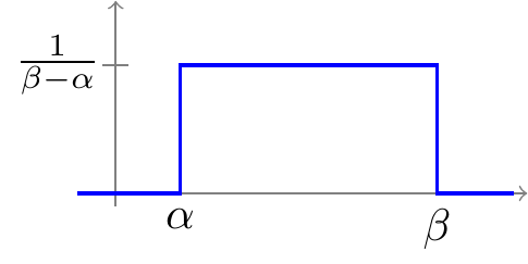
Definition 22.1 (Uniform distribution) A random variable \(X\) is said to have a \(\text{Uniform}(a, b)\) distribution if its PDF is
\[ f(x) = \begin{cases} \frac{1}{b - a} & a < x < b \\ 0 & \text{otherwise} \end{cases}. \tag{22.1}\]
This PDF is graphed below:
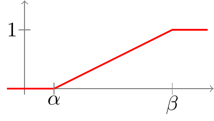
Equivalently, a random variable has a \(\text{Uniform}(a, b)\) distribution if its CDF is \[ F(x) = \int_{-\infty}^x f(t)\,dt = \begin{cases} 0 & x \leq a \\ \frac{x-a}{b-a} & a < x < b \\ 1 & x \geq b \end{cases}.\]
This CDF is graphed below.
Using Definition 22.1, the distance \(X\) of one of
Joyner-Kersee’s long jumps is a \(\textrm{Uniform}(a= 6.3, b= 7.5)\) random variable. We can use the PDF or CDF to calculate probabilities such as \(P(7.0 < X < 7.3)\).
In fact, R has a built-in function for the CDF of a uniform distribution, punif, which we can use to calculate probabilities. For example, to determine \(P(7.0 < X < 7.3)\), we can calculate \(F(7.3) - F(7.0)\) in R as follows:
We can derive any uniform distribution as a location-scale transformation of the standard uniform distribution—that is, a \(\textrm{Uniform}(a= 0, b= 1)\) distribution. To see this, let \(U\) be a standard uniform random variable. If we scale \(U\) by \((b - a)\) and shift by \(a\), then the resulting variable will be uniformly distributed between \(a\) and \(b\).
22.1.1 Expectation and Variance
Proposition 22.1 provides a simple way to derive the expectation and variance of any uniform distribution. First, we calculate the expectation \(\text{E}\!\left[ U \right]\) and variance \(\text{Var}\!\left[ U \right]\) for a standard uniform random variable \(U\). Then, we use properties of expected value and variance for linear transformations to derive the expectation of a general uniform random variable.
Using Proposition 22.2, it is easy to calculate that the expected distance of one of Joyner-Kersee’s long jumps is \[\text{E}\!\left[ X \right] = \frac{6.3 + 7.5}{2},\] and the variance of one of her long jumps is \[\text{Var}\!\left[ X \right] = \frac{(7.5 - 6.3)^2}{12} = 0.12.\]
22.2 Exponential
The exponential distribution is used to model the time until some event. In Example 18.7, we used this distribution to model the time until the first click of a Geiger counter.
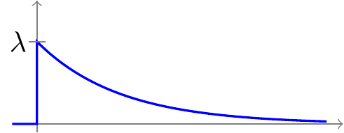
Definition 22.2 (Exponential Distribution) A random variable \(X\) is said to have a \(\text{Exponential}(\lambda)\) distribution if its PDF is
\[ f(x) = \begin{cases} \lambda e^{-\lambda x} & x > 0 \\ 0 & \text{otherwise} \end{cases}, \tag{22.2}\]
where \(\lambda\) is the rate at which events occur.
This PDF is graphed below:
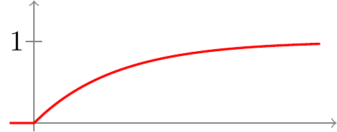
Equivalently, a random variable has a \(\text{Exponential}(\lambda)\) distribution if its CDF is \[ F(x) = \int_{-\infty}^x f(t)\,dt = \begin{cases} 0 & x \leq 0 \\ 1 - e^{-\lambda x} & x > 0 \end{cases}.\]
This CDF is graphed below.
In this language, we can describe the time (in seconds) until the first click of a Geiger counter from Example 18.7, \(T\), as an \(\textrm{Exponential}(\lambda=1.2)\) random variable. We can use the PDF or CDF to calculate probabilities such as \(P(T > 2.3)\).
In fact, R has a built-in function for the CDF of an exponential distribution, pexp, which we can use to calculate probabilities. For example, to determine \(P(T > 2.3)\), we can calculate \(1 - F(2.3)\) in R as follows:
We can derive any exponential distribution as a scale transformation of the standard exponential distribution—that is, a \(\textrm{Exponential}(\lambda=1)\) distribution. To see this, let \(Z\) be a standard exponential random variable. Note that \(Z\) is measured in time units so that the rate is \(1\). To convert back to the original time units, we need to scale \(Z\) by \(\frac{1}{\lambda}\).
22.2.1 Expectation and Variance
Proposition 22.3 provides a simple way to derive the expectation and variance of any exponential distribution. First, we calculate the expectation \(\text{E}\!\left[ Z \right]\) and variance \(\text{Var}\!\left[ Z \right]\) for a standard exponential random variable \(Z\). Then, we use properties of expected value and variance for linear transformations to derive the expectation of a general exponential random variable.
Using Proposition 22.4, it is easy to write down the expected time of the first click of the Geiger counter from Example 18.7: \[\text{E}\!\left[ X \right] = \frac{1}{\lambda} = \frac{1}{2.6},\] and the variance of the time of the first click: \[\text{Var}\!\left[ X \right] = \frac{1}{\lambda^2} = \frac{1}{2.6^2}.\]
22.2.2 Memoryless Property
The exponential distribution is frequently used to model the time until an event. What are some practical implications of using the exponential model?
One property of the exponential distribution is that it is memoryless. That is, if the event has not happened by time \(t\), then the remaining time until the event happens has the same exponential distribution.
The memoryless property is controversial. In real-world situations, we expect that if you have already waited a long time, then the remaining waiting time will be shorter. But when we use the exponential distribution to model waiting times, this will not be the case because of the memoryless proeprty. For this reason, statisticians and engineers typically use non-memoryless distributions, such as the Weibull distribution, to model waiting times.
22.3 Normal
The normal distribution is the most important continuous model in probability and statistics. In Example 18.5, we used the normal distribution to model the high temperature in May in Iqaluit.
To begin our formal discussion of the normal distribution, we will first define the standard normal distribution, which is a bell-shaped PDF centered around \(0\). Then, we will apply location-scale transformations to the standard normal distribution to construct general normal distributions, which are bell-shaped PDFs that can have any width and be centered around values other than \(0\).
22.3.1 Standard Normal Distribution
Unfortunately, this integral is not easy to evaluate because \(e^{-x^2 / 2}\) has no elementary antiderivative. We can approximate the integral numerically using R.
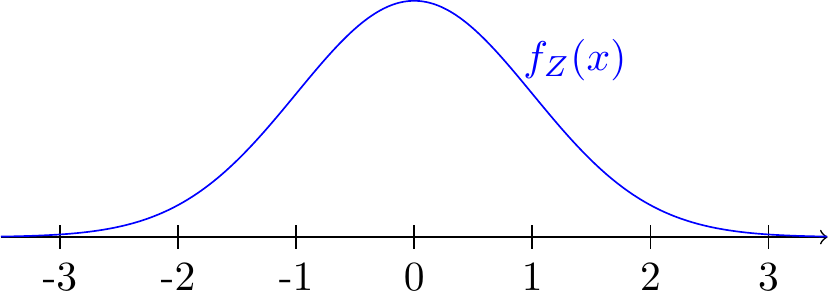
In Example 23.9, we will use tools from joint distributions to show that \(k = \sqrt{2\pi}\) so that the standard normal PDF is \[ \begin{equation} f(x) = \frac{1}{\sqrt{2\pi}} e^{-x^2 / 2}; \qquad -\infty < x < \infty. \end{equation} \tag{22.4}\]
This PDF is graphed in Figure 22.5.
Equivalently, a random variable has a standard normal distribution if its CDF is \[ \Phi(x) \overset{\text{def}}{=}\int_{-\infty}^x \frac{1}{\sqrt{2\pi}} e^{-t^2/2}\,dt. \tag{22.5}\]
Because the PDF Equation 22.4 has no elementary antiderivative, the CDF cannot be simplified beyond Equation 22.5. For this reason, we will often express probabilities in terms of the standard normal CDF \(\Phi\). Note that we are using the symbol \(\Phi\) for the standard normal CDF, as opposed to the more generic \(F\). This is an indication of the importance of the standard normal CDF.
Example 22.1 Let \(Z\) be a standard normal random variable. What is \(P(-2 < Z < 2)\)?
This probability corresponds to the red shaded area below.
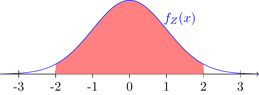
We can express this probability in terms of the CDF \(\Phi\).
\[ \begin{align} P(-2 < Z < 2) &= P(Z \leq 2) - P(Z \leq -2) \\ &= \Phi(2) - \Phi(-2) \\ \end{align} \tag{22.6}\]
Because the standard normal curve is symmetric around 0, it must be the case that \[ \begin{aligned} P(Z > 2) &= P(Z < -2) \\ 1 - \Phi(2) &= \Phi(-2). \end{aligned} \] Substituting this into Equation 22.6, we obtain the equivalent expression \[ P(-2 < Z < 2) = \Phi(2) - (1 - \Phi(2)) = 2\Phi(2) - 1.\]
In order to evaluate this probability numerically, we use the pnorm function in R, which corresponds to \(\Phi\). The two lines of code below should produce the same answer, based on our calculations above.
The probability is about 95%.
Following the same procedure, we can show that
- \(P(-1 < Z < 1) = \Phi(1) - \Phi(-1) \approx 68\%\),
- \(P(-2 < Z < 2) = \Phi(2) - \Phi(-2) \approx 95\%\), and
- \(P(-3 < Z < 3) = \Phi(3) - \Phi(-3) \approx 99.7\%\),
leading to the 68-95-99.7 rule for calculating normal probabilities. This rule is helpful for approximating probabilities numerically when a standard normal CDF calculator (like R) is not available. For example, if we wanted to approximate \(P(Z \geq 2.5)\), we could observe that this probability is somewhere between \(P(Z \geq 3)\) and \(P(Z \geq 2)\), which we can obtain using the 68-95-99.7 rule.
A lower bound for this probability is \[ \begin{aligned} P(Z \geq 3) &= \frac{1}{2} P(|Z| \geq 3) & \text{(symmetry)} \\ &= \frac{1}{2}(1 - P(-3 < Z < 3)) & \text{(complement rule)} \\ &\approx \frac{1}{2}(1 - .997) & \text{(68-95-99.7 rule)} \\ &= .0015, \end{aligned} \] and a similar calculation shows an upper bound to be \(P(Z \geq 2) \approx .025\). Therefore, \(P(Z \geq 2.5)\) should be somewhere between 0.15% and 2.50%.
Since we have a calculator handy, we can check this approximation by evaluating \(P(Z \geq 2.5) = 1 - \Phi(2.5)\) to high precision.
22.3.2 General Normal Distribution
The general normal distribution is defined as a location-scale transformation of a standard normal distribution. That is, the general normal PDF is bell-shaped, like the standard normal PDF (Equation 22.4), but with a different width and centered around a value that is not necessarily \(0\).
However, we do not usually have to work with Equation 22.8 because we can always convert a normal random variable into a standard normal random variable, by a process called standardization. Standardization is simply the inverse of Equation 22.7. It says that \[ Z = \frac{X - \mu}{\sigma}. \tag{22.9}\] The next example illustrates how standardization can be used to solve problems.
22.3.3 Expectation and Variance
Because we defined the (general) normal distribution as a location-scale transformation of a standard normal random variable, we can derive the expectation and variance easily. First, we calculate the expectation \(\text{E}\!\left[ Z \right]\) and variance \(\text{Var}\!\left[ Z \right]\) for a standard uniform random variable \(Z\). Then, we use Proposition 21.2 and Proposition 21.3 to obtain the expectation and variance of a general normal random variable.