48 Confidence Intervals

In this book so far, we have focused mostly on point estimation, where the goal is to produce a single estimate of a parameter of interest, ignoring the uncertainty in this estimate. In this chapter, we will discuss how to report a range of plausible values of a parameter, capturing the uncertainty in our estimate. This range of values is called a confidence interval and has a fundamental connection with the hypothesis tests from Chapter 47.

48.1 The \(z\)-interval

Recall Example 47.1, where the quality engineers take daily samples of \(n=5\) ball bearings from a production line. One day, the diameters of the ball bearings (in mm) are measured to be \[ X_1 = 10.06, X_2 = 10.07, X_3 = 9.98, X_4 = 10.02, X_5 = 10.09. \] It is assumed that \(X_1, \dots, X_5\) are i.i.d. \(\text{Normal}(\mu, \sigma^2 = 0.03^2)\).

In Example 47.1, we tested whether the production line was producing ball bearings that met the specification of \(\mu = 10\) mm. Alternatively, we can estimate \(\mu\), the mean diameter of ball bearings currently being produced by the line.

We know from Example 30.3 that the maximum likelihood estimate of \(\mu\) is \[ \bar X = 10.044. \]

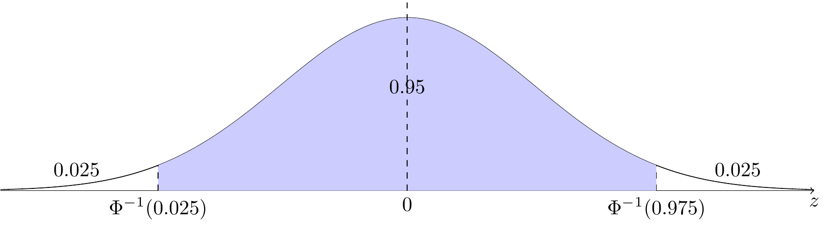
This is a point estimate of \(\mu\). We can quantify the uncertainty by reporting a 95% confidence interval. To do so, first observe that \[ Z = \frac{\bar X - \mu}{\sqrt{\sigma^2 / n}} \tag{48.1}\] is standard normal, so by definition, \[ P(\Phi^{-1}(0.025) < Z < \Phi^{-1}(0.975)) = 0.95. \] This is illustrated in Figure 48.1. (Note that \(\Phi^{-1}(0.975) = -\Phi^{-1}(0.025) \approx 1.96 \approx 2\).)

Figure 48.1: The probability that \(Z\) lies between \(\Phi^{-1}(0.025)\) and \(\Phi^{-1}(0.975)\) is \(0.95\)

Substituting Equation 48.1 for \(Z\), we can rearrange the inequalities so that \(\mu\) is in the middle: \[ \begin{align} &P\left(\Phi^{-1}(0.025) \leq \frac{\bar X - \mu}{\sqrt{\sigma^2 / n}} \leq \Phi^{-1}(0.975)\right) \\ &= P\left(\Phi^{-1}(0.025) \sqrt{\frac{\sigma^2}{n}} \leq \bar X - \mu \leq \Phi^{-1}(0.975)\sqrt{\frac{\sigma^2}{n}} \right) \\ &= P\left(\bar X - \Phi^{-1}(0.025)\sqrt{\frac{\sigma^2}{n}} \geq \mu \geq \bar X - \Phi^{-1}(0.975)\sqrt{\frac{\sigma^2}{n}}\right). \end{align} \]

This leads to the conclusion that the random interval \[ \left[\bar X - \Phi^{-1}(0.975) \sqrt{\frac{\sigma^2}{n}}, \bar X - \Phi^{-1}(0.025) \sqrt{\frac{\sigma^2}{n}}\right] \] has a 95% probability of containing \(\mu\). This is called a 95% confidence interval for \(\mu\).

For the ball bearings data, a 95% confidence interval for \(\mu\) is \[ \left[10.044 - 1.96 \sqrt{\frac{0.03^2}{5}}, 10.044 + 1.96 \sqrt{\frac{0.03^2}{5}}\right] = [10.0177, 10.0703]. \tag{48.2}\] We say that we are 95% confident that \(\mu\) is between \(10.0177\) mm and \(10.0703\) mm.

We cannot say for certain whether \(\mu\) is between these two numbers or not, but we know that an interval constructed in this way will contain \(\mu\) 95% of the time. We can illustrate this via simulation. For the simulation, we have to assume a particular value of \(\mu\).

About 95% of these intervals contain \(\mu = 10.02\) in this simulation. In practice, we only ever observe one of these intervals, and we have no way of knowing whether \(\mu\) is in that interval or not. However, we hope that our interval is one of 95% of intervals that do contain \(\mu\), as opposed to the 5% that do not.

The next proposition summarizes the results of this section, generalizing them to confidence levels other than 95%.

Proposition 48.1 (\(z\)-interval for a normal mean) Let \(X_1, \dots, X_n\) be i.i.d. \(\text{Normal}(\mu, \sigma^2)\) random variables, where \(\sigma^2\) is known.

A \((1-\alpha)\) confidence interval for \(\mu\) is \[ \left[\bar X - \Phi^{-1}(1 - \alpha/2) \sqrt{\frac{\sigma^2}{n}}, \bar X - \Phi^{-1}(\alpha/2) \sqrt{\frac{\sigma^2}{n}} \right] = \bar X \pm \Phi^{-1}(1 - \alpha/2) \sqrt{\frac{\sigma^2}{n}}. \] Notice that we used the symmetry of the normal distribution to conclude that \(\Phi^{-1}(\alpha / 2) = -\Phi^{-1}(1 - \alpha/2)\). This allows us to write the confidence interval as \(\bar X \pm \Phi^{-1}(1 - \alpha/2) \sqrt{\frac{\sigma^2}{n}}\).

In the rest of this chapter, we will focus on the case where \(\alpha = 0.05\) (95% confidence intervals), although it is straightforward to generalize the results to other values of \(\alpha\).

48.2 Duality of Confidence Intervals and Hypothesis Tests

The 95% confidence interval that we constructed in Equation 48.2 did not contain \(\mu = 10.00\), which agrees with our decision in Example 47.1 to reject the null hypothesis that \(\mu = 10.00\). This is no coincidence. A 95% confidence interval will contain exactly the values of \(\mu\) that are not rejected by the corresponding hypothesis test.

Proposition 48.2 (Duality of confidence intervals and hypothesis tests) Suppose that a hypothesis test of \(H_0: \theta = \theta_0\) rejects when \[ \vec X \in R(\theta_0) \] for some rejection region \(R(\theta_0)\), defined so that the \(p\)-value is 5% when the null hypothesis is true: \[ P_{\theta_0}(\vec X \in R(\theta_0)) = 0.05. \] (The notation \(P_{\theta_0}\) simply reminds us that the probability is calculated assuming that \(\vec X\) comes from a distribution where \(\theta = \theta_0\).)

Then, \(C(\vec X) \overset{\text{def}}{=}\{ \theta: \vec X \notin R(\theta) \}\) is a 95% confidence set for \(\theta\). (Although \(C(\vec X)\) will be an interval in all the cases we will consider, there is no guarantee that it will be an interval, so we refer to \(C(\vec X)\) as a confidence set just to be safe.)

Proof

For every \(\theta_0\), we have \[ \begin{align} P_{\theta_0}(\theta_0 \in C(\vec X)) &= P_{\theta_0}(\vec X \notin R(\theta_0)) \\ &= 1 - P_{\theta_0}(\vec X \in R(\theta_0)) \\ &= 0.95. \end{align} \]

Proposition 48.2 says that we can “invert” a hypothesis test to obtain a confidence interval and vice versa. If we invert the \(z\)-test from Section 47.1, then we obtain the \(z\)-interval above.

Example 48.1 (Duality of the \(z\)-test and the \(z\)-interval) The \(z\)-test from Section 47.1 rejects the null hypothesis \(H_0: \mu = \mu_0\) when \[ |Z| = \left| \frac{\bar X - \mu_0}{\sqrt{\sigma^2 / n}} \right| > \Phi^{-1}(0.975). \]

In other words, this test does not reject when \[ \Phi^{-1}(0.025) \leq \frac{\bar X - \mu_0}{\sqrt{\sigma^2 / n}} \leq \Phi^{-1}(0.975). \]

If we solve for the values of \(\mu_0\) for which the test does not reject, we obtain \[ \bar X - \Phi^{-1}(0.025)\sqrt{\frac{\sigma^2}{n}} \geq \mu_0 \geq \bar X - \Phi^{-1}(0.975)\sqrt{\frac{\sigma^2}{n}}, \] which is precisely the \(z\)-interval from Section 48.1.

48.3 The \(t\)-interval

In the examples so far, we assumed the variance \(\sigma^2\) was known. What if it is not known?

In Section 47.2, we saw that for hypothesis testing, we can perform a \(t\)-test instead of a \(z\)-test. In the \(t\)-test, we replace \(\sigma^2\) by the sample variance \(S^2\). This introduces additional uncertainty, so instead of comparing to a standard normal distribution, we compare to a \(t\)-distribution.

We can use Proposition 48.2 to invert the \(t\)-test to obtain a confidence interval when \(\sigma^2\) is unknown. The result is called a \(t\)-interval.

Proposition 48.3 (\(t\)-interval for a normal mean) Let \(X_1, \dots, X_n\) be i.i.d. \(\text{Normal}(\mu, \sigma^2)\) random variables, where \(\sigma^2\) is unknown.

A 95% confidence interval for a mean \(\mu\) is \[ \left[\bar X - F_{t_{n-1}}^{-1}(0.975) \sqrt{\frac{S^2}{n}}, \bar X - F_{t_{n-1}}^{-1}(0.025) \sqrt{\frac{S^2}{n}} \right] = \bar X \pm F_{t_{n-1}}^{-1}(0.975) \sqrt{\frac{S^2}{n}}, \] where \(F_{t_{n-1}}\) is the CDF of a \(t\)-distribution with \(n-1\) degrees of freedom and \(S^2\) is the sample variance (Definition 38.1).

Proof

The \(t\)-test from Section 47.2 rejects the null hypothesis \(H_0: \mu = \mu_0\) when \[ |T| = \left| \frac{\bar X - \mu_0}{\sqrt{S^2 / n}} \right| > F_{t_{n-1}}^{-1}(0.975). \] That is, the \(t\)-test compares the \(t\)-statistic to a \(t\)-distribution.

In other words, this test does not reject when \[ F_{t_{n-1}}^{-1}(0.025) \leq \frac{\bar X - \mu_0}{\sqrt{S^2 / n}} \leq F_{t_{n-1}}^{-1}(0.975). \]

If we solve for the values of \(\mu_0\) for which the test does not reject, we obtain \[ \bar X - F_{t_{n-1}}^{-1}(0.025)\sqrt{\frac{S^2}{n}} \geq \mu_0 \geq \bar X - F_{t_{n-1}}^{-1}(0.975)\sqrt{\frac{S^2}{n}}, \] which corresponds to the interval above.

Armed with the \(t\)-interval, we can calculate a 95% confidence interval for the average human body temperature.

Example 48.2 (Confidence interval for the average human body temperature) In Example 47.2, we concluded that the average human body temperature is not \(98.6^\circ\text{F}\), but what is it? We can use the data to form a 95% confidence interval.

In the examples that we have encountered so far, we started with a function of the data and the parameter, \[ g(\vec X; \theta), \tag{48.3}\] whose distribution is known and does not depend on \(\theta\). This is called a pivot (or pivotal quantity). In the examples above, the pivots were

\(Z = \frac{\bar X - \mu}{\sqrt{\frac{\sigma^2}{n}}}\) follows a standard normal distribution.
\(T = \frac{\bar X - \mu}{\sqrt{\frac{S^2}{n}}}\) follows a \(t\)-distribution with \(n-1\) degrees of freedom.

To obtain a confidence interval for \(\theta\), we used the quantiles of the pivot’s known distribution and rearranged the inequality.

48.4 Asymptotic Confidence Intervals

If \(X_1, \dots, X_n\) are not i.i.d. normal, then it is not easy to obtain a pivot. In these situations, it may not be possible to obtain a confidence interval with exactly 95% probability of covering \(\mu\). However, we can still obtain an interval with approximate 95% coverage when \(n\) is large, thanks to the Central Limit Theorem.

Proposition 48.4 (Wald intervals) Let \(X_1, \dots, X_n\) be i.i.d. random variables with mean \(\mu\). Then, \[ Z \overset{\text{def}}{=}\frac{\bar X - \mu}{\sqrt{\sigma^2 / n}} \] is asymptotically standard normal by the Central Limit Theorem (Theorem 36.1). Therefore, the interval \[ \bar X \pm \Phi^{-1}(0.975) \sqrt{\frac{\sigma^2}{n}} \] has coverage \[ \begin{align} &P\left(\bar X - \Phi^{-1}(0.025)\sqrt{\frac{\sigma^2}{n}} \geq \mu \geq \bar X - \Phi^{-1}(0.975)\sqrt{\frac{\sigma^2}{n}}\right)\\ &= P(\Phi^{-1}(0.025) \leq Z \leq \Phi^{-1}(0.975)) \\ &\approx 0.95. \end{align} \]

If \(\sigma^2\) is unknown, then we can replace it with any consistent estimate \(\hat\sigma^2\) (such as the sample variance \(S^2\)), in which case \[ Z' \overset{\text{def}}{=}\frac{\bar X - \mu}{\sqrt{\hat\sigma^2 / n}} = \frac{\frac{\bar X - \mu}{\sqrt{\sigma^2 / n}}}{\sqrt{\hat\sigma^2 / \sigma^2}} \overset{d}{\to} \frac{Z}{1} \] by Slutsky’s theorem (see Theorem 37.3). Therefore, the interval \[ \bar X \pm \Phi^{-1}(0.975) \sqrt{\frac{\hat\sigma^2}{n}} \] also has approximate 95% coverage.

These asymptotic confidence intervals are known as Wald intervals. We now return to the skew die example that we encountered at the beginning of our exploration of statistical inference in Chapter 29 and construct a Wald interval for the probability \(p\) of rolling a six.

Example 48.3 (Wald interval for a binomial proportion) In Example 29.4, we rolled a skew die \(n = 25\) times and observed that six came up exactly \(X = 7\) times. Can we use this information to come up with a confidence interval for \(p\), the probability of rolling a six? We already know that the MLE of \(p\) is \(\hat p = \frac{7}{25} = 0.28\).

If we express \(X\) as a sum of Bernoulli random variables \(I_1 + \dots + I_n\), then we see that \[ \hat p = \frac{X}{n} = \frac{I_1 + \dots + I_n}{n} = \bar I \] and \(\mu = \text{E}\!\left[ I_1 \right] = p\). Therefore, we can use Proposition 48.4 to construct an approximate confidence interval for \(p\).

Since we do not know \(\sigma^2 = \text{Var}\!\left[ I_1 \right] = p(1 - p)\), we will estimate it by \(\hat\sigma^2 = \hat p(1 - \hat p)\), which is consistent for \(\sigma^2\) by the continuous mapping theorem (Theorem 37.2). (This turns out to be equivalent to the sample variance \(S^2\) of the Bernoulli random variables.)

Now, Proposition 48.4 says that the interval \[ \begin{align} \hat p \pm \Phi^{-1}(0.975) \sqrt{\frac{\hat p (1 - \hat p)}{n}} &\approx 0.28 \pm 1.96 \sqrt{\frac{0.28 (1 - 0.28)}{25}} \\ &\approx [0.104, 0.456] \end{align} \] is an approximate 95% confidence interval for \(p\).

The Wald interval is only guaranteed to have 95% coverage as \(n\to\infty\). How good is the interval for \(n=25\)? We can answer this question by simulation. To do this, we have to assume a particular value of \(p\).

Shockingly, a 95% Wald interval only covers \(p = 0.12\) about 81% of the time. Notice in particular that when \(\hat p = 0\), the Wald interval is \([0, 0]\), which seems awfully pessimistic. This example illustrates the dangers of relying on asymptotic results.

We can obtain an interval with better coverage by returning to first principles (Proposition 48.2). We start by deriving a test of \(H_0: p = p_0\). Then, we invert this test to obtain a confidence interval.

Example 48.4 (Wilson interval for a binomial proportion) An asymptotic test of \(H_0: p = p_0\) does not reject when \[ \Phi^{-1}(0.025) \leq \underbrace{\frac{\hat p - p_0}{\sqrt{p_0(1-p_0) / n}}}_{Z} \leq \Phi^{-1}(0.975). \] Notice that \(p_0\) appears in both the numerator and denominator of \(Z\) because we are using the exact mean and variance of \(\hat p\) under the null hypothesis.

To invert this test, we need to solve for \(p_0\), which is more difficult because \(p_0\) appears in both the numerator and denominator. First, we square both sides to obtain \[ \frac{(\hat p - p_0)^2}{p_0(1-p_0) / n} \leq \Phi^{-1}(0.975)^2. \]

This can be rearranged into a quadratic inequality in \(p_0\): \[ \begin{align} (\hat p - p_0)^2 - \frac{\Phi^{-1}(0.975)^2}{n} p_0(1-p_0) &\leq 0 \\ \left(1 + \frac{\Phi^{-1}(0.975)^2}{n}\right)p_0^2 - \left(2\hat p + \frac{\Phi^{-1}(0.975)^2}{n}\right) p_0 + \hat p^2 &\leq 0, \end{align} \] which is satisfied for \(p_0\) lying between the roots of the quadratic. Using the quadratic formula, the above inequality is equivalent to the interval \[ \begin{align} & \frac{1}{1 + \frac{\Phi^{-1}(0.975)^2}{n}} \left( \left(\hat p + \frac{\Phi^{-1}(0.975)^2}{2n}\right) \pm \sqrt{\left(\hat p + \frac{\Phi^{-1}(0.975)^2}{2n} \right)^2 - \left( 1 + \frac{\Phi^{-1}(0.975)^2}{n} \right) \hat p^2} \right) \\ &= \frac{1}{1 + \frac{\Phi^{-1}(0.975)^2}{n}} \left( \left(\hat p + \frac{\Phi^{-1}(0.975)^2}{2n}\right) \pm \Phi^{-1}(0.975) \sqrt{\frac{\hat p (1 - \hat p)}{n} + \frac{\Phi^{-1}(0.975)^2}{4n^2}} \right). \end{align} \]

Applying this to the skew die example, we obtain the Wilson interval \[ \begin{align} \frac{1}{1 + \frac{1.96^2}{25}} \left( \left(0.28 + \frac{1.96^2}{2(25)} \right) \pm 1.96 \sqrt{\frac{0.28 (1 - 0.28)}{25} + \frac{1.96^2}{4(25)^2}}\right) &\approx \frac{1}{1.1537} \left( 0.3568 \pm 0.1920 \right) \\ &= [0.143, 0.476]. \end{align} \]

This is called the Wilson interval for the binomial proportion. Comparing it with the Wald interval from Example 48.3, we see that:

the Wilson interval is scaled by \(\frac{1}{1 + \frac{\Phi^{-1}(0.975)^2}{n}}\),
the Wilson interval is centered around \(\hat p + \frac{\Phi^{-1}(0.975)^2}{2n}\) instead of \(\hat p\), and
the Wilson interval estimates \(\text{Var}\!\left[ \hat p \right]\) by \(\frac{\hat p (1 - \hat p)}{n} + \frac{\Phi^{-1}(0.975)^2}{4n^2}\) instead of \(\frac{\hat p (1 - \hat p)}{n}\).

All of these adjustments become negligible as \(n\to\infty\), which makes sense because the Wald interval has asymptotic 95% coverage. Nevertheless, these small adjustments improve the coverage dramatically for finite \(n\), as the simulation below demonstrates.

Whereas the coverage of the Wald interval was 81%, the coverage of the Wilson interval is close to 95%! Furthermore, unlike the Wald interval, the Wilson interval gives a sensible answer when \(\hat p = 0\): \[ \left[0, \frac{\Phi^{-1}(0.975)^2}{n + \Phi^{-1}(0.975)^2}\right], \] which results in the interval \([0, 0.133]\) for the example above.

The Wilson interval is still asymptotic; it relies on the Central Limit Theorem and is only guaranteed to have 95% coverage as \(n \to \infty\). However, because it was derived by inverting a hypothesis test that used the exact variance \(\sigma^2 = p_0 (1 - p_0)\) instead of an estimate, it tends to perform much better than the Wald interval for smaller values of \(n\).

48.5 Exercises

Exercise 48.1 (Confidence interval for an exponential mean) Let \(X_1, \dots, X_n\) be i.i.d. \(\text{Exponential}(\lambda)\). Consider forming a confidence interval for \(\mu \overset{\text{def}}{=}1/\lambda\).

Form a 95% Wald interval for \(\mu\).
Form a 95% confidence interval for \(\mu\) by deriving a test of \(H_0: \mu = \mu_0\) and inverting the test.
Compare the coverage of the two intervals using simulation.