26  From Conditionals to Marginals

$$

$$

In Chapter 16, we considered situations where the distribution of two discrete random variables \(X\) and \(Y\) was specified by

1. first specifying the PMF of \(X\),
2. then specifying the conditional PMF of \(Y\) given \(X\).

We saw that the (marginal) PMF of \(Y\) could be calculated using the Law of Total Probability (Theorem 7.1) \[ f_Y(y) = \sum_x f(x, y) = \sum_x f_X(x) f_{Y|X}(y|x). \tag{26.1}\]

We now generalize Equation 26.1 to the situation where \(X\) or \(Y\) may be continuous.

26.1 Laws of Total Probability

As a warm-up, we revisit Example 23.7, where \(X\) and \(Y\) represent the times that you and a friend have to wait to enter an amusement park. We assumed that \(X\) and \(Y\) were independent \(\text{Exponential}(\lambda_1)\) and \(\text{Exponential}(\lambda_2)\) random variables, respectively. Previously, we calculated \(P(X < Y)\) using a double integral. Now, we show how to calculate this probability using the Law of Total Probability.

Example 26.1 (Queueing theory (Law of Total Probability version)) If we condition on the event \(\{ X = x \}\), then we obtain a probability that involves only one random variable: \[ P(X < Y | X = x) = P(Y > x | X = x) = P(Y > x). \] We can calculate this latter probability by integrating the PDF of \(Y\), or using its known CDF: \[ P(Y > x) = 1 - F_Y(x) = 1 - (1 - e^{-\lambda_2 x}) = e^{-\lambda_2 x}. \]

Now, we aggregate these conditional probabilities to obtain the overall probability of \(\{ X < Y \}\). To do this, we use the continuous analog of the Law of Total Probability. \[ P(X < Y) = \int_{-\infty}^\infty P(X < Y | X = x) f_X(x)\,dx. \tag{26.2}\] Equation 26.2 is just like its discrete cousin, except with the PMF replaced by the PDF and the sum replaced by an integral.

Now, we calculate \[ \begin{align} P(X < Y) &= \int_{-\infty}^\infty P(X < Y | X = x) f_X(x)\,dx \\ &= \int_{0}^\infty e^{-\lambda_2 x} \lambda_1 e^{-\lambda_1 x}\,dx \\ &= \lambda_1 \int_{0}^\infty e^{-(\lambda_1 + \lambda_2) x} \,dx \\ &= \frac{\lambda_1}{\lambda_1 + \lambda_2}, \end{align} \] which matches the answer that we obtained using a double integral in Example 23.7.

Example 26.1 reinforces a point we made after Example 23.7. Double integrals are rarely the most intuitive way to solve most real problems in probability and statistics. If you think carefully about the structure of a problem, you can usually avoid double integrals (or calculus altogether)!

Now, we are ready to state the general version of the Law of Total Probability. In fact, there are many versions, depending on whether \(X\) and \(Y\) are discrete or continuous.

Proposition 26.1 (Law(s) of Total Probability) Let \(X\) and \(Y\) be random variables.

1. If \(X\) is a discrete random variable with PMF \(f_X(x)\), then the PMF or PDF of \(Y\) (depending on whether \(Y\) is discrete or continuous, respectively) is given \[ f_Y(y) = \sum_x f_X(x) f_{Y|X}(y|x). \tag{26.3}\]
2. If \(X\) is a continuous random variable with PDF \(f_X(x)\), then the PMF or PDF of \(Y\) (depending on whether \(Y\) is discrete or continuous, respectively) is described by \[ f_Y(y) = \int_{-\infty}^\infty f_X(x) f_{Y|X}(y|x)\,dx. \tag{26.4}\]

Note that \(f_{Y|X}(y|x)\) denotes a conditional PMF or PDF, depending on whether \(Y\) is discrete or continuous, respectively.

In Chapter 16, we saw several applications of Proposition 26.1 when \(X\) and \(Y\) are both discrete. So we focus on the other possibilities in the examples below. In the first example, the random variable we are conditioning on, \(I\), is discrete, so Equation 26.3 applies.

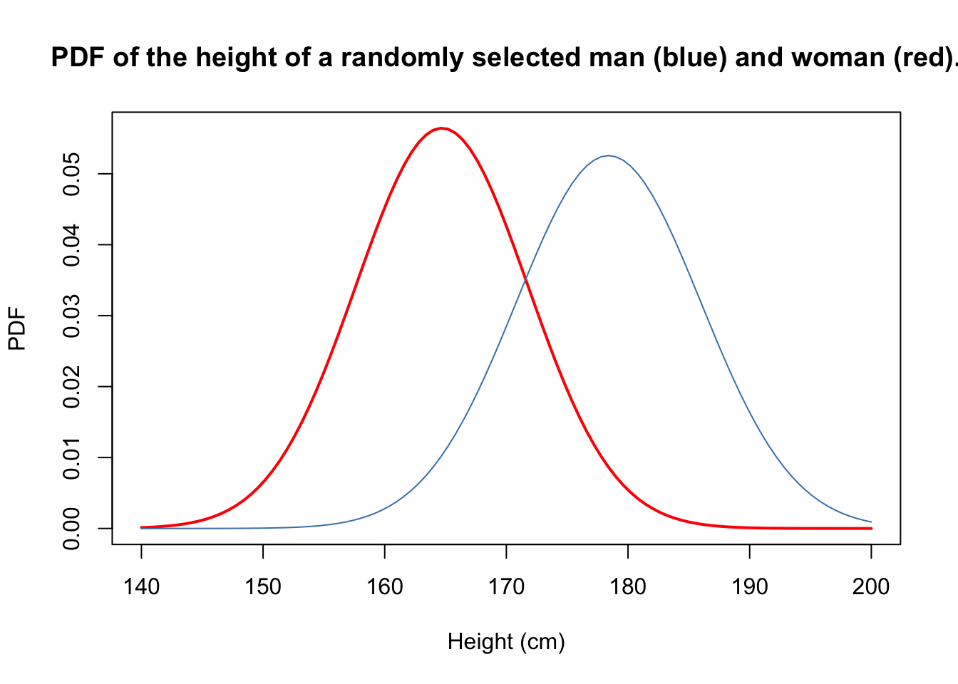
Example 26.2 (Sexual dimorphism) In biology, sexual dimorphism refers to morphological differences between males and females of the same species. One common example is human height. Data shows that the heights of adult human males and females are approximately normally distributed, but with different means and variances. (Jelenkovic et al. 2016)

Let \(I\) be an indicator variable for the event that a randomly selected person is female. Then the height \(H\) of the selected adult has the following conditional distributions:

\[ \begin{align} H \mid \{ I = 0 \} &\sim \textrm{Normal}(\mu= 178.4 \text{ cm}, \sigma^2= 7.59^2 \text{ cm}^2) \\ H \mid \{ I = 1 \} &\sim \textrm{Normal}(\mu= 164.7 \text{ cm}, \sigma^2= 7.07^2 \text{ cm}^2). \end{align} \]

These distributions are graphed below.

Human populations tend to be skewed towards males: \[ f_I(0) = P(I = 0) = 0.51, \quad f_I(0) = P(I = 1) = 0.49. \]

The general Law of Total Probability (Proposition 26.1) says that the marginal PDF of \(H\) is \[\begin{align*} f_H(h) &\approx f_I(0) \cdot f_{H \mid I}(h \mid 0) + f_I(1) \cdot f_{H \mid I}(h \mid 1) \\ &= 0.51 \cdot \frac{1}{\sqrt{2\pi \cdot 7.59^2}} \exp\left( -\frac{(h - 178.4)^2}{2 \cdot 7.59^2} \right) \\ &\quad + 0.49 \cdot \frac{1}{\sqrt{2\pi \cdot 7.07^2}} \exp\left( -\frac{(h - 164.7)^2}{2 \cdot 7.07^2} \right). \end{align*}\] Note that \(H\) is continuous, so both \(f_H(h)\) and \(f_{H\mid I}(h\mid i)\) are PDFs.

The figure below shows what the PDF of \(H\) looks like.

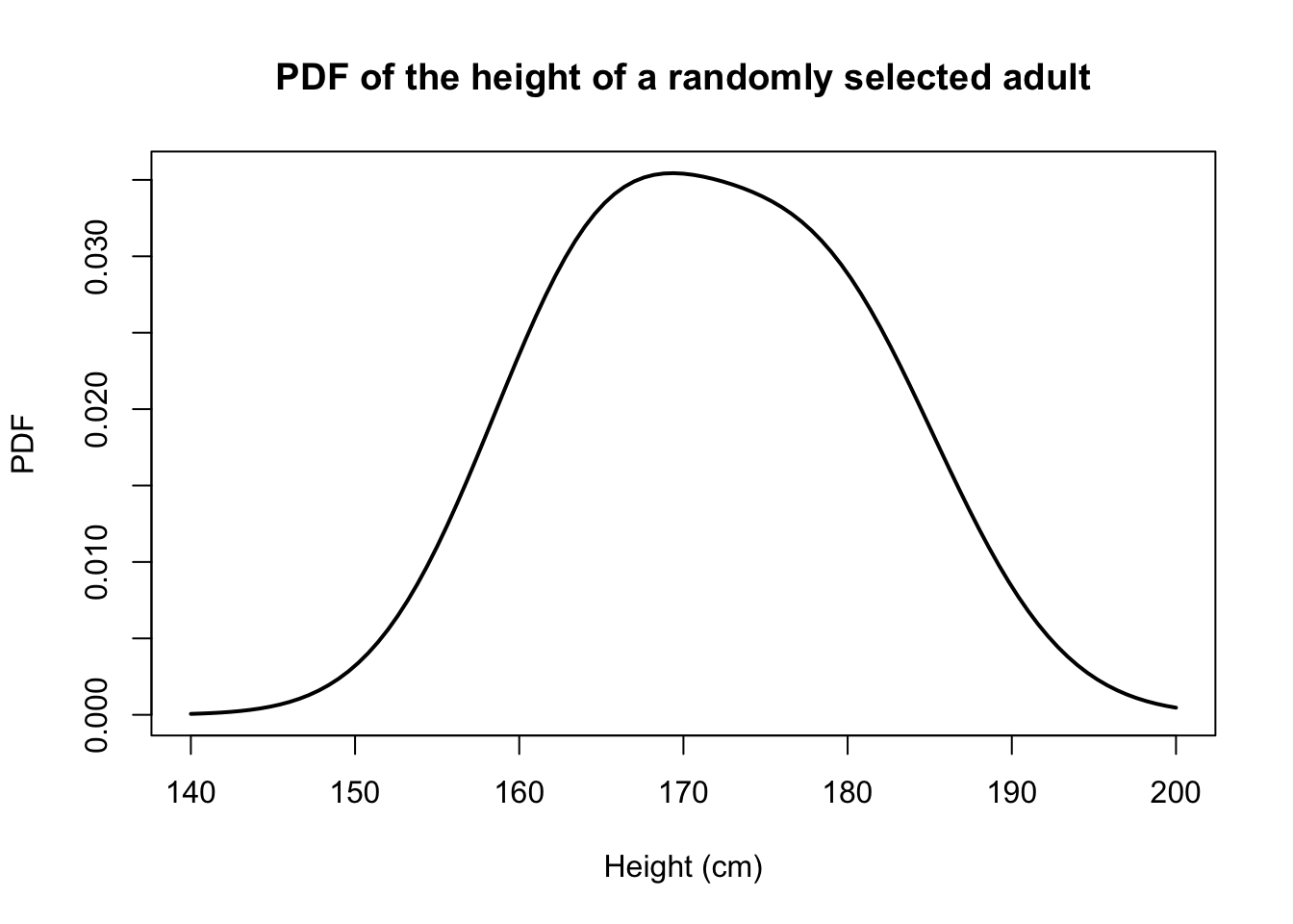
Notice that this distribution is not normal. Instead, it is a mixture of two different normal distributions.

In the next example, the random variable we are conditioning on, \(S\), is discrete, so Equation 26.4 applies.

Example 26.3 (Free throws in basketball) A person is chosen at random from the population and asked to shoot \(n\) basketball free throws. Let \(X\) be the number of free throws that person makes. What is the distribution of \(X\)?

Each person has a different probability of making a free throw, depending on their skill. Since the person is chosen at random, this skill is a random variable \(S\). Suppose we model \(S\) as a \(\textrm{Uniform}(a= 0, b= 1)\) random variable. (All skill levels are equally likely.)

Conditional on \(S\), it seems reasonable to assume that the \(n\) free throws are independent, so \[ X | \{ S = s \} \sim \text{Binomial}(n, p=s). \]

But what is the marginal distribution of \(X\)? We can use the Law of Total Probability, conditioning on the skill \(S\) of the person we selected: \[ \begin{align} f_X(x) &= \int_{-\infty}^\infty f_S(s) f_{X|S}(x|s)\,ds \\ &= \int_0^1 1 \cdot \binom{n}{x} s^x (1 - s)^{n-x} \,ds; & x=0, 1, \dots, n. \end{align} \tag{26.5}\] Note that \(X\) is discrete, so both \(f_X(x)\) and \(f_{X\mid S}(x\mid s)\) are PMFs.

This integral is a polynomial in \(s\), so it is straightforward to evaluate for any particular values of \(n\) and \(x\). However, it is not obvious how to devise a general formula.

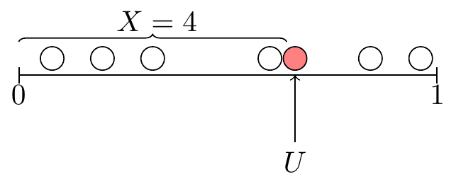
In the same paper that introduced Bayes’ rule, Thomas Bayes (1763) devised a clever way to evaluate Equation 26.5. He imagined \(n+1\) balls being rolled across a table. (Later writers interpreted these to be billiards balls on a pool table.) Suppose that each of these balls is equally likely to land anywhere on the opposite side, independently of the other balls. If the opposite side has length \(1\), then the position of the balls are independent \(\textrm{Uniform}(a= 0, b= 1)\) random variables. To map this situation onto the model above,

• let \(S\) be the position of the initial ball, and
• let \(X\) be the number of the remaining \(n\) balls that lie to the left of the initial ball. Conditional on the position of the initial ball \(\{ S = s \}\), each ball has a probability \(s\) of being to the left, and the balls are independent by assumption. Therefore, \(X | \{ S = s\}\) is binomial.

This situation is illustrated in Figure 26.1 for \(n=6\).

Figure 26.1: Illustration of Bayes’ billiards balls, with the initial ball highlighted in red.

What is the marginal distribution of \(X\)? Since the \(n+1\) balls are identical, they are all equally likely to be the initial ball. If the initial ball is the leftmost ball, then \(X = 0\); if it is the rightmost ball, then \(X = n\); all values in between are equally likely. Therefore, \[ f_X(x) = \frac{1}{n+1}; \qquad x=0, 1, \dots, n. \tag{26.6}\]

If Bayes’ argument seems too clever, we will see a more straightforward way to show that the integral in Equation 26.5 is equal to Equation 26.6 in Chapter 41, after developing more machinery.

26.2 Bayes’ Rule

Recall from Theorem 7.2 that Bayes’ rule allows us to compute \(P(B \mid A)\) from \(P(A \mid B)\). Bayes’ rule can be generalized to random variables; it allows us to determine the distribution of \(X \mid Y\) from the distribution of \(Y \mid X\).

Proposition 26.2 (Bayes’ rule for random variables) Let \(X\) and \(Y\) be random variables. Then,

\[ f_{X \mid Y}(x \mid y) = \frac{f_X(x) f_{Y \mid X}(y \mid x)}{f_Y(y)}, \tag{26.7}\]

where \(f_X\), \(f_Y\), \(f_{X \mid Y}\) and \(f_{Y \mid X}\) are PMFs or PDFs, depending on whether \(X\) and \(Y\) are discrete or continuous.

Proof

We will prove this for the case where \(X\) and \(Y\) are both continuous. The case where \(X\) and \(Y\) are both discrete is already covered by Theorem 7.2. The case where \(X\) is discrete and \(Y\) is continuous (or vice versa) is beyond the scope of this book.

We can expand the joint PDF in two ways: \[ f_{X, Y}(x, y) = f_Y(y) f_{X \mid Y}(x|y) = f_X(x) f_{Y \mid X}(y|x). \] Dividing both sides by \(f_Y(y)\), we obtain Equation 26.7.

Proposition 26.2 is especially useful when one random variable is observable, but the other is not. For example, in Example 26.3, it is easy to observe \(X\), the number of free throws made, but it is difficult to observe \(S\), the skill of the person taking the free throws. In this case, we can use Bayes’ rule to make inferences about \(S\), given \(X\).

Example 26.4 (Inferring skill from free throws) Continuing with Example 26.3, suppose the randomly selected person shoots \(n = 18\) free throws and makes \(X = 12\) of them. What can we infer about their skill \(S\)?

Before we watched this person take free throws, \(S\) was equally likely to be \(0\) and \(1\). This is our prior belief about their skill level. In light of the information that they made two-thirds of their \(18\) free throws, we should update our belief about their skill.

To make this precise, we determine the conditional PDF of \(S\) given \(X\) via Proposition 26.2.

\[ \begin{align} f_{S|X}(s|x) &= \frac{f_S(s) f_{X|S}(x|s)}{f_X(x)} \\ &= \frac{1 \cdot \binom{n}{x} s^x(1-s)^{n-x}}{\frac{1}{n+1}} \\ &= (n+1) \binom{n}{x} s^x (1 - s)^{n-x} \end{align} \] for \(0 < s < 1\) and \(x = 0, 1, \dots n\).

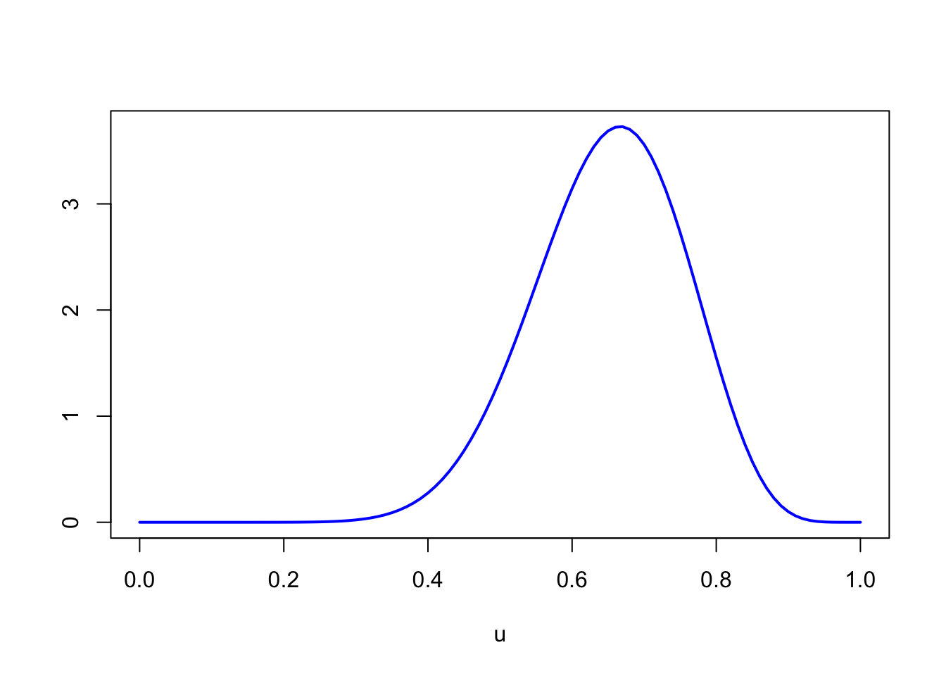
Substituting in \(n=18\) and \(x=12\), the conditional distribution of \(S\) is \[ f_{S|X}(s|12) = 19 \binom{18}{12} s^{12} (1 - s)^6; \qquad 0 < s < 1. \]

This PDF is graphed below. This represents our updated, or posterior, belief about their skill level, as a result of the observed data.

Figure 26.2: Conditional PDF of \(S\) given \(X = 12\)

Example 26.5 (Inferring gender from height) Returning to Example 26.2, suppose we randomly select a person who is \(182.9 \text{ cm}\) tall (i.e., approximately \(6 \text{ ft}\)). What is the probability that they are female?

To find this probability, we use the general Bayes’ rule (Proposition 26.2) to compute \(P(I = 1 | H = 182.9)\):

\[\begin{align*} &P(I = 1 \mid H =182.9) & \\ &= f_{I \mid H}(1 \mid 182.9) & \\ &= \frac{f_I(1) \cdot f_{H \mid I}(182.9 \mid 1)}{f_H(182.9)} & \\ &\approx \frac{0.49 \cdot \frac{1}{\sqrt{2\pi \cdot 7.07^2}} \exp\left( -\frac{(182.9 - 164.7)^2}{2 \cdot 7.07^2} \right)}{ 0.49 \cdot \frac{1}{\sqrt{2\pi \cdot 7.07^2}} \exp\left( -\frac{(182.9 - 164.7)^2}{2 \cdot 7.07^2} \right) + 0.51 \cdot \frac{1}{\sqrt{2\pi \cdot 7.59^2}} \exp\left( -\frac{(182.9 - 178.4)^2}{2 \cdot 7.59^2} \right)} & \\ &\approx 0.043 & \end{align*}\]

The probability that a \(182.9 \text{ cm}\) tall person is a woman is only about \(0.043\).

Bayes, Thomas. 1763. “An Essay Towards Solving a Problem in the Doctrine of Chances.” Philosophical Transactions of the Royal Society of London, no. 53: 370–418.

Jelenkovic, Aline, Yoon-Mi Hur, Reijo Sund, Yoshie Yokoyama, Sisira H Siribaddana, Matthew Hotopf, Athula Sumathipala, et al. 2016. “Genetic and Environmental Influences on Adult Human Height Across Birth Cohorts from 1886 to 1994.” eLife 5 (December): e20320. https://doi.org/10.7554/eLife.20320.