29  Probability versus Statistics

Although probability is a fascinating subject in its own right, it is perhaps most important in the modern world because of its application to statistics. In this chapter, we discuss the intricate relationship between probability and statistics.

29.1 Mark-Recapture

We introduced mark-recapture in Example 12.3 as a method for estimating the size of a population, such as the number of snails in a state park. First, we capture a sample, say \(50\) snails, and “mark” them. Then, after some time, we recapture another sample of snails, say \(40\). Some of these snails will be marked from the first capture, while the rest are unmarked. In Chapter 12, we learned to solve probability problems like the following.

Example 12.3 (Mark-Recapture as a Probability Problem)

Suppose there are actually \(300\) snails in the population. What is the probability that exactly \(11\) marked snails are recaptured in the second sample of \(40\) snails?

If every snail in the population has an equal chance of being sampled, then the number of marked snails in the second sample, \(X\), is a \(\text{Hypergeometric}(n=40, M=50, N=300)\) random variable, and we can calculate the probability of exactly \(11\) marked snails by substituting \(x = 11\) into the hypergeometric PMF (Equation 12.2): \[ P(X = 11) = f_{40, 50, 300}(11) = \frac{\binom{50}{11} \binom{250}{29}}{\binom{300}{40}} \approx .0276. \]

We can also use R to evaluate this probability:

But Example 12.3 is unrealistic. If we knew that there were \(300\) snails in the population, we would not bother doing mark-recapture in the first place!

Here is a more realistic problem, where we have collected data and want to infer something about the population.

Example 29.1 (Mark-Recapture as a Statistics Problem) Suppose that \(X = 11\) of the recaptured snails are marked. What can we infer about \(N\), the number of snails in the population?

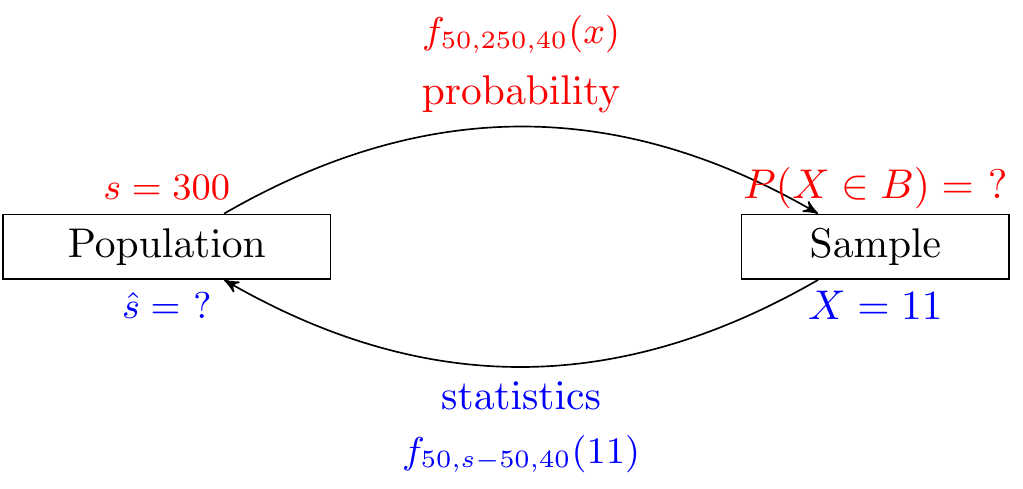
In Example 12.3, we assumed that \(N = 300\) and wanted to calculate the probabilities of various values of \(X\), whereas in Example 29.1, we observe \(X = 11\) and want to estimate \(N\). In other words, statistics is the inverse of probability. This idea is illustrated in Figure 29.1.

Figure 29.1: Relationship between probability and statistics for mark-recapture. Note that \(f(x)\) denotes the hypergeometric PMF.

Properties of the population (or model), such as \(N\), are called parameters, while properties of the sample (or data), such as \(X\), are called statistics. How do we estimate a parameter using data? The probability distribution still plays an important role. However, the unknown quantity is now the parameter \(N\), instead of the value of the random variable \(X\). This motivates the following definition:

Definition 29.1 (Likelihood) Let \(f_\theta(x)\) be a PMF (or PDF) with parameter(s) \(\theta\). The likelihood of \(\theta\) is defined as \[ L_x(\theta) = f_\theta(x). \]

In other words, the likelihood is simply the PMF (or PDF) regarded as a function of the unknown parameter \(\theta\), instead of \(x\).

Let us determine the likelihood for the mark-recapture problem.

Example 29.2 (Mark-Recapture Likelihood) If \(X = 11\) of the recaptured snails are marked, then the likelihood of \(N\) is \[ L_{11}(N) = f_{40, 50, 300}(11) = \frac{\binom{50}{11} \binom{N-50}{29}}{\binom{N}{40}}. \] In other words, the likelihood represents \(P(X = 11)\) for different values of \(N\).

We can graph the likelihood as follows:

How do we use the likelihood to estimate \(N\)? Since the likelihood represents the probability of observing the data, one idea is to choose \(N\) to make this probability as large as possible. This principle is stated below.

Definition 29.2 (Principle of Maximum Likelihood) One way to estimate a parameter \(\theta\) is to choose the value of \(\theta\) that maximizes the likelihood. That is,

\[ \hat\theta = \arg\max_\theta L_x(\theta). \]

This value is called the maximum likelihood estimate (or MLE).

To find the MLE for the mark-recapture problem, we find the value of \(N\) that maximizes \(L_{11}(N)\). From Example 29.2, we see that the likelihood is maximized somewhere between 150 and 200. To determine the exact value, we print out the likelihood for all values of \(N\) between 150 and 200.

We see that the likelihood is maximized at \(N = 181\), where it achieves a maximum value of \(0.15854\). Therefore, the MLE for the size of the snail population is \(\hat N = 181\). This value makes intuitive sense. The data suggests that approximately \(11 / 40 = 0.275\) of all snails are marked. Since we marked \(50\) snails, the number of snails in the population should be \(50 / 0.275 \approx 181.82\), which is very close to the MLE.

This is no accident. We can derive the MLE as a function of the number of marked snails \(M\), the number of snails in the second sample \(n\), and and the number of marked snails \(x\). To do this, we consider the ratio \(L_x(N) / L_x(N - 1)\):

\[ \begin{align} \frac{L_x(N)}{L_x(N - 1)} &= \frac{\frac{\binom{M}{x} \binom{N - M}{n - x}}{\binom{N}{n}}}{\frac{\binom{M}{x} \binom{N - 1 - M}{n - x}}{\binom{N - 1}{n}}} \\ &= \frac{(N - n)(N - M)}{N(N - M - n + x)}. \end{align} \]

The likelihood is increasing if and only if this ratio is greater than \(1\)—that is, when \[ \begin{align*} (N - n)(N - M) &> N(N - M - n + x) \\ N^2 - NM - nN + nM &> N^2 - NM - nN + Nx \\ nM &> Nx. \end{align*} \] In other words, the likelihood will increase as long as \(N < \frac{nM}{x}\), and it will decrease when \(N > \frac{nM}{x}\). Therefore, the likelihood is maximized when \(N\) is the greatest integer not exceeding \(\frac{nM}{x}\): \[ \hat N = \left\lfloor \frac{nM}{x} \right\rfloor. \]

This captures the intuition that the best estimate of the population size is the value of \(N\) that makes \(\frac{M}{N} \approx \frac{x}{n}\).

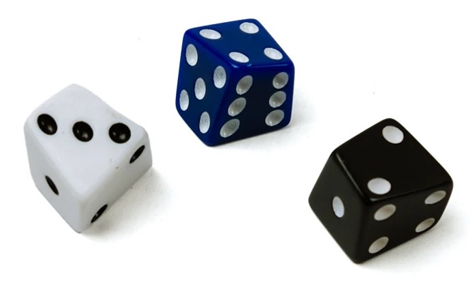
29.2 Skew Dice

A skew die is one whose faces are irregular. Are skew dice fair? One way to find out is to roll the die and collect some data.

You should already be familiar with how to solve problems like the following.

Example 29.3 (Skew Dice as a Probability Problem) Suppose that a skew die has a probability \(p = 0.18\) of landing on a six. If the die is rolled 25 times, what is the probability that six comes up exactly 7 times?

Assuming that the dice rolls are independent, the number of sixes is a \(\text{Binomial}(n=25, p=0.18)\) random variable \(X\). Let \(f_{n, p}(x)\) be the PMF. Then, \[ P(X = 7) = f_{25, 0.18}(7) = \binom{25}{7} (0.18)^{7} (1 - 0.18)^{18} \approx .0827. \]

We can also use R to evaluate this probability:

But the whole point of rolling the die is to determine the probability of landing on each face. That is, the statistics question is likely more compelling than the probability question.

Figure 29.2: Relationship between probability and statistics for skew dice. Note that \(f(x)\) denotes the binomial PMF.

Example 29.4 (Skew Dice as a Statistics Problem) Suppose that a skew die is rolled 25 times and six comes up exactly 7 times. What can we infer about the probability \(p\) that this die lands on a six?

We can use maximum likelihood. The likelihood of \(p\) based on this data is \[ L_7(p) = f_{25, p}(7) = \binom{25}{7} p^7 (1 - p)^{18}. \]

We graph this likelihood below. Note that \(p\) is a continuous parameter; it can take on any value between \(0\) and \(1\).

Where is this likelihood maximized? Because \(p\) is a continuous parameter, we can maximize \(L_7(p)\) by taking the derivative and setting it equal to 0:

\[ \begin{align} 0 &= \frac{d}{dp} L_7(p) \\ &= \frac{d}{dp} \binom{25}{7} p^7 (1 - p)^{18} \\ &= \binom{25}{7} \big(7p^6 (1 - p)^{18} - 18 p^7 (1 - p)^{17}\big) \\ &= \binom{25}{7} p^6 (1 - p)^{17} \big(7(1 - p) - 18p\big) \end{align} \]

There are three solutions to this equation: \(p = 0, 1, \frac{7}{25}\). The first two correspond to minima, so the MLE is \[ \hat p = \frac{7}{25} = 0.28. \]

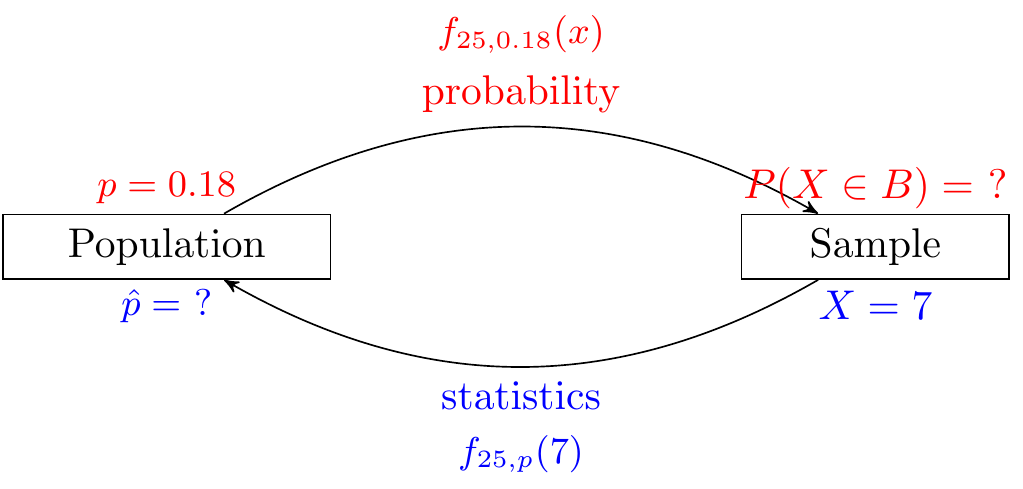
The MLE in Example 29.4 is intuitive. If the skew die landed on six \(7\) times in \(25\) rolls, then our best estimate for the probability of landing on six is \(\frac{7}{25}\). We can show this fact more generally, by replacing \(25\) by \(n\) and \(7\) by \(x\).

The likelihood of \(p\) is \[ L_x(p) = \binom{n}{x} p^x (1 - p)^{n - x}. \] Taking the derivative again with respect to \(p\), we obtain \[ \begin{align} 0 &= \frac{\partial}{\partial p} L_x(p) \\ &= \frac{\partial}{\partial p} \binom{n}{x} p^x (1 - p)^{n - x} \\ &= \binom{n}{x} \big(x p^{x - 1} (1 - p)^{n - x} - (n - x) p^x (1 - p)^{n - x - 1}\big) \\ &= \binom{n}{x} p^{x - 1} (1 - p)^{n - x - 1} \big(x (1 - p) - (n - x) p\big). \end{align} \] The solution to this equation corresponding to a maximum is \[ \hat p = \frac{x}{n}. \]

29.3 Exercises

Exercise 29.1 Suppose \(X\) is a discrete random variable with \(P(X = 7) = p\) and \(P(X = 8) = 1-p\). Three independent observations are made: \(x_1 = 7\), \(x_2 = 8\), and \(x_3 = 7\). What is the MLE of \(p\)?

Exercise 29.2 (Geometric MLE) Let \(X \sim \text{Geometric}(p)\). Suppose we observe \(X = x\). What is the MLE of \(p\) (in terms of \(x\))?

Exercise 29.3 (Poisson MLE) Let \(X \sim \text{Poisson}(\mu)\). Suppose we observe \(X = x\). What is the MLE of \(\mu\) (in terms of \(x\))?

Exercise 29.4 (MLE of the number of trials) Suppose you toss a coin \(n\) times, but you lose track of how many times you flipped the coin. However, you know the coin has a probability \(p\) of landing heads, and you recall counting \(k\) heads. What is the MLE of \(n\)?

Exercise 29.5 (Simple random sampling) You are interested in the proportion of students at a university who own a dog. Suppose that there are \(N = 7500\) students at the university, and you randomly ask \(n = 130\) students (without replacement) whether or not they own a dog. This is called a simple random sample of size \(n\) from the population (of size \(N\)).

You find that \(X = 60\) of the \(n = 130\) students in your sample own a dog. Based on this information, what is the MLE of \(p\), the proportion of students who own a dog?

Hint: If \(M\) is the number of students at the university who own a dog, then \(p = \frac{M}{N}\). It may help to find the MLE of \(M\) first. You can do this using R or using algebra, as in Section 29.1.

Exercise 29.6 (Hardy-Weinberg principle) The Hardy-Weinberg principle predicts the frequency of genetic variants in a population in equilibrium.

For example, in the MN blood group system, there are two alleles, M and N, so each person’s blood type is either MM, MN, or NN. If \(p\) is the frequency of allele M (and \(1 - p\) is the frequency of allele N), then the Hardy-Weinberg principle predicts that the three blood types occur with the following frequencies:

MM	MN	NN
\(p^2\)	\(2p(1 - p)\)	\((1 - p)^2\)

In a sample of \(n=1029\) people from the Chinese population of Hong Kong in 1937, it was observed that the blood types occurred in the following frequencies.

MM	MN	NN
\(342\)	\(500\)	\(187\)

Using this data, calculate the maximum likelihood of \(p\), the frequency of allele M in the Chinese population of Hong Kong.