36 Central Limit Theorem

In Chapter 33, we saw that the exact distribution of the sample mean $\bar X_n$ of i.i.d. exponential random variables is difficult to derive using convolutions. Unfortunately, moment generating functions are not much help either (Example 34.8). However, we can still derive accurate approximations to the distribution of $\bar X_n$ when $n$ is large.

In this chapter, we apply the theory from Chapter 35 to derive the asymptotic distribution of the sum and mean of i.i.d. random variables. Before we dive into the theory, we first illustrate the result using simulations.

Example 36.1 (Mean of i.i.d. exponential random variables) Let $X_1, \dots, X_n$ be i.i.d. $\text{Exponential}(\lambda)$. We saw that the MLE of $\mu = 1/\lambda$ is $\bar X_n = \sum_{i=1}^n X_i$. What is its sampling distribution?

The code below simulates the sum of $n$ independent exponential random variables, assuming $\lambda = 0.5$. Try increasing the value of n in the code below. What happens to the distribution of the sum as $n$ increases?

Example 36.2 (Sum of i.i.d. Poisson random variables) Let $X_1, \dots, X_n$ be i.i.d. $\textrm{Poisson}(\mu=1)$. What is the distribution of $\sum_{i=1}^n X_i$? The code below simulates the sum of $n$ independent Poisson random variables. Try increasing the value of n in the code below. What happens to the distribution of the sum as $n$ increases?

In both examples above, we saw that distribution approached a normal distribution as $n\to\infty$. This is no accident: the mean or the sum of i.i.d. random variables with (essentially) any distribution will be asymptotically normal! This result, which explains the ubiquity of the normal distribution in nature, is known as the Central Limit Theorem.

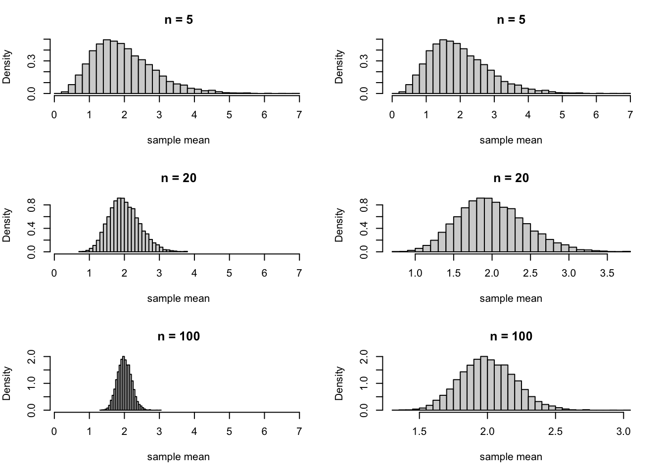
To make the statement precise, we revisit the case where $X_1, X_2, \dots$ are i.i.d. $\textrm{Poisson}(\mu=1)$ random variables. We know that $\bar X_n$ converges in distribution to $\mu$. This is represented by the left column of Figure 36.1. As $n\to\infty$, the distribution collapses to a point mass at $\mu = 1$.

Figure 36.1: Simulated values of $\bar X_n$ for $n=5, 20, 100$, where $X_1, X_2, \dots$ are i.i.d. $\textrm{Exponential}(\lambda=0.5)$. In the left column, the $x$-axis is held fixed, while in the right column, we zoom in on the $x$-axis as $n$ increases.

However, if we zoom in at just the right rate, we can see that the distribution of $\bar X_n$ around the mean $\mu = 2$ is approximately normal. This is represented by the right column of Figure 36.1. To make this precise, we will consider the limiting distribution of \[ Y_n \overset{\text{def}}{=}\sqrt{n} (\bar X_n - \mu). \tag{36.1}\]

We know that $\bar X_n - \mu \stackrel{d}{\to} 0$, but if we zoom in at a rate of $\sqrt{n}$, then the resulting distribution will be nondegenerate. To see why $\sqrt{n}$ is the right rate, consider the variance: \[ \text{Var}\!\left[ Y_n \right] = \text{Var}\!\left[ \sqrt{n} (\bar X_n - \mu) \right] = n \text{Var}\!\left[ \bar X_n \right] = n \cdot \frac{\sigma^2}{n} = \sigma^2, \] where $\sigma^2 \overset{\text{def}}{=}\text{Var}\!\left[ X_1 \right]$. In other words, $\sqrt{n}$ is exactly the right rate to ensure that the variance neither diverges to $\infty$, nor collapses to $0$.

Notice that Equation 36.1 can also be written in terms of the sum: \[ Y_n = \frac{1}{\sqrt{n}} \sum_{i=1}^n (X_i - \mu). \tag{36.2}\]

It turns out that this form of $Y_n$ is more convenient for proving the Central Limit Theorem, but this expression is identical to Equation 36.1.

36.1 Statement and Proof

To find the limiting distribution of $Y_n$, we will use MGFs and Theorem 35.3.

Theorem 36.1 (Central Limit Theorem) Let $X_1, X_2, \dots$ be a sequence of i.i.d. random variables with mean $\mu\overset{\text{def}}{=}\text{E}\!\left[ X_1 \right]$ and variance $\sigma^2 \overset{\text{def}}{=}\text{Var}\!\left[ X_1 \right]$. Then, \[ Y_n \overset{\text{def}}{=}\frac{1}{\sqrt{n}} \sum_{i=1}^n (X_i - \mu) \stackrel{d}{\to} \text{Normal}(0, \sigma^2). \]

Proof

We will prove Theorem 36.1 under the assumption that $X_1, X_2, \dots$ have a moment generating function in an interval containing $0$, although this is not necessary. A more general proof would use characteristic functions (Equation 34.5), which are guaranteed to exist.

If we define $W_i \overset{\text{def}}{=}X_i - \mu$, then \[ Y_n = \frac{1}{\sqrt{n}} \sum_{i=1}^n W_i. \] The MGF of $Y_n$ is \[ M_{Y_n}(t) = \text{E}\!\left[ e^{\frac{t}{\sqrt{n}} \sum_{i=1}^n W_i} \right] = \text{E}\!\left[ e^{\frac{t}{\sqrt{n}} W_1} \right]^n = M_{ W_1}\left(\frac{t}{\sqrt{n}}\right)^n \]

Now, we take the limit as $n\to\infty$. To make the algebra easier, we take logs and reparametrize in terms of $\delta \overset{\text{def}}{=}\frac{t}{\sqrt{n}}$: \[ \begin{align} \log M_{Y_n}(t) &= n \log M_{W_1}\left(\frac{t}{\sqrt{n}}\right) \\ &= \frac{t^2}{\delta^2} \log M_{W_1}(\delta). \end{align} \] Now, we take the limit as $\delta \to 0$. Along the way, we will need the derivatives of the MGF of $W_1$ at $0$:

$M_{W_1}(0) = 1$ (since $\text{E}\!\left[ e^{0} \right] = 1$)
$M_{W_1}'(0) = \text{E}\!\left[ W_1 \right] = 0$ (since $\text{E}\!\left[ W_1 \right] = \text{E}\!\left[ X_1 - \mu \right] = \mu - \mu$)
$M_{W_1}''(0) = \text{E}\!\left[ {W_1}^2 \right] = \text{Var}\!\left[ X_1 \right] = \sigma^2$ (since $\text{E}\!\left[ W_1^2 \right] = \text{E}\!\left[ (X_1 - \mu)^2 \right] = \text{Var}\!\left[ X_1 \right]$).

\[ \begin{align} \lim_{n\to\infty} \log M_{Y_n}(t) &= t^2 \lim_{\delta \to 0} \frac{\log M_{W_1}(\delta)}{\delta^2} & (\text{indeterminate form $0/0$}) \\ &= t^2 \lim_{\delta \to 0} \frac{\frac{M'_{W_1}(\delta)}{M_{W_1}(\delta)}}{ 2\delta } & (\text{L'H\^{o}pital's rule}) \\ &= t^2 \lim_{\delta \to 0} \frac{M'_{W_1}(\delta)}{ 2\delta } \underbrace{\lim_{\delta\to 0} \frac{1}{M_{W_1}(\delta)}}_{1} & \text{(properties of limits)} \\ &= t^2 \lim_{\delta \to 0} \frac{M''_{W_1}(\delta)}{2} & (\text{L'H\^{o}pital again}) \\ &= \frac{t^2 \sigma^2}{2}. \end{align} \]

Now, undoing the log transformation, this implies that \[ M_{Y_n}(t) \to e^{\frac{t^2 \sigma^2}{2}}. \] This limit is the MGF of the $\text{Normal}(0, \sigma^2)$ distribution from Example 34.2. Therefore, by Theorem 35.3, \[ Y_n = \frac{1}{\sqrt{n}} \sum_{i=1}^n (X_i - \mu) \stackrel{d}{\to} \text{Normal}(0, \sigma^2). \]

Notice that the calculation in this proof was essentially identical to Example 35.1.

The Central Limit Theorem (or CLT, for short) is remarkable. We made no assumptions about the distribution of $X_1$, other than that it has finite mean and variance. Although we assumed that $X_1, X_2, \dots$ are i.i.d., there are other versions of the Central Limit Theorem that allow the random variables to be dependent (but not too dependent) and to have different distributions (but not too different). Because the Central Limit Theorem holds under such general settings, it explains the ubiquity of the normal distribution in nature, a point illustrated by the following video.

36.2 Applications

The Central Limit Theorem (CLT) can be used to obtain approximate answers to a wide variety of problems. In fact, we have already encountered one example.

Example 36.3 (Normal approximation to the binomial revisited) In Example 35.1, we approximated $X_n \sim \text{Binomial}(n, p)$ by a $\textrm{Normal}(\mu= np, \sigma^2= np(1-p))$ distribution. Although we derived this approximation from scratch, it is in fact a special case of the Central Limit Theorem.

By Example 14.3, we know that \[ X_n = I_1 + I_2 + \dots + I_n, \] where $I_1, I_2, \dots, I_n$ are i.i.d. $\text{Bernoulli}(p)$ random variables. Theorem 36.1 says that \[ \frac{X_n - np}{\sqrt{n}} = \frac{1}{\sqrt{n}} \sum_{k=1}^{n} (I_k - p) \stackrel{\cdot}{\sim} \textrm{Normal}(\mu= 0, \sigma^2= p(1-p)). \] which matches the result we derived in Example 35.1. (Recall that the dot over $\sim$ indicates that this is an asymptotic distribution.)

The practical consequence of the Central Limit Theorem is that the distribution of a sum or a mean of a large number $n$ of i.i.d. random variables can be approximated by a normal distribution with the same mean and variance. That is,

\[ S_n \overset{\text{def}}{=}\sum_{i=1}^n X_i \stackrel{\cdot}{\sim} \text{Normal}(n\mu, n\sigma^2) \tag{36.3}\] \[ \bar{X}_n \overset{\text{def}}{=}\frac{1}{n} S_n \stackrel{\cdot}{\sim} \text{Normal}(\mu, \frac{\sigma^2}{n}), \tag{36.4}\]

where $\mu \overset{\text{def}}{=}\text{E}\!\left[ X_1 \right]$ and $\sigma^2 \overset{\text{def}}{=}\text{Var}\!\left[ X_1 \right]$ are the mean and variance of an individual random variable in the sum.

In the next example, we use the Central Limit Theorem to explain the phenomenon seen in Figure 36.1.

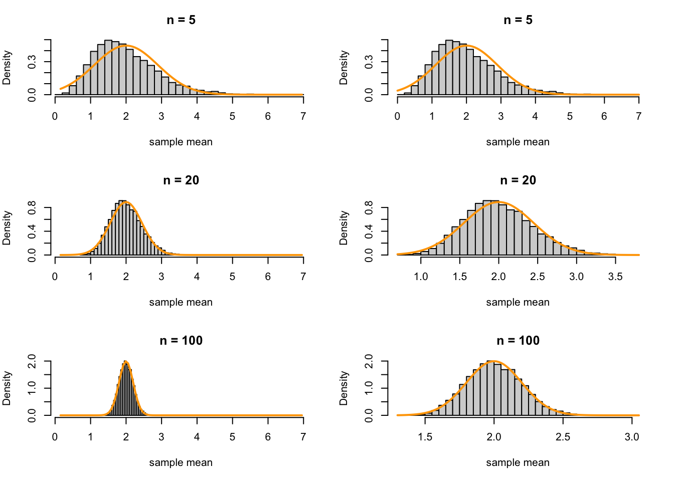
Example 36.4 (Asymptotic distribution of the MLE of the exponential mean) In Example 36.1, we saw that the distribution of the sample mean $\bar X_n$ of i.i.d. $\text{Exponential}(\lambda)$ random variables is approximately normal.

By Equation 36.4, we know that \[ \bar{X}_n \stackrel{\cdot}{\sim} \textrm{Normal}(\mu= \frac{1}{\lambda}, \sigma^2= \frac{1}{n\lambda^2}), \]

Adding this PDF to the simulations from Figure 36.1 for $\lambda = 0.5$, we see that the approximation is poor for $n=5$, better for $n=20$, and very good (but still not perfect) for $n=100$.

At the end of Chapter 33, we calculated the probability that $\bar X_2$ and $\bar X_3$ were within 10% of the true mean of $\mu = 1 / \lambda$; even for $n=3$, the probability was only about $0.13$. Now, we can use the normal approximation to do the same for $\textcolor{orange}{\bar X_{100}}$. \[ \begin{align} P(0.9\mu < \textcolor{orange}{\bar X_{100}} < 1.1\mu) &= P\Bigg( \frac{0.9\mu - \mu}{\sqrt{\frac{\mu^2}{100}}} < \underbrace{\frac{\textcolor{orange}{\bar X_{100}} - \mu}{\sqrt{\frac{\mu^2}{100}}}}_{Z} < \frac{1.1\mu - \mu}{\sqrt{\frac{\mu^2}{100}}} \Bigg) \\ &= \Phi\left(\frac{1.1 - 1}{\sqrt{\frac{1}{100}}}\right) - \Phi\left(\frac{0.9 - 1}{\sqrt{\frac{1}{100}}}\right) \\ &\approx 0.6827. \end{align} \]

The probability that the sample mean is within 10% of $\mu$ exceeds $0.68$ when $n = 100$. By the Law of Large Numbers, we know that this probability will approach $1$ as $n\to\infty$.

In the last example, we show that the CLT can be useful, even when dealing with a random variable that is neither a sum nor a mean.

Example 36.5 (Binomial model in finance) The binomial model is a simple but popular model for stock prices. In this model, at each time step, the price of a stock either increases by a factor $u$ (with probability $p$) or decreases by a factor $d$ (with probability $1-p$). The changes in price at each time step are assumed to be independent.

For example, consider a stock that starts at $s_0$, and suppose that each day, the price of the stock has a $p=0.6$ chance of increasing by 2% or decreases by 2%. That is, the changes in the stock price are i.i.d. random variables $X_1, X_2, \dots$ with PMF

$x$	$0.98$	$1.02$
$f(x)$	$0.4$	$0.6$

Now, the price of the stock after $n$ days is \[ S_n = s_0 \prod_{i=1}^n X_i. \]

At first, it may not seem like the Central Limit Theorem applies here because $S_n$ is the product of many random variables, not the sum. However, if we take logs, then we obtain \[ \log \frac{S_n}{s_0} = \sum_{i=1}^n \log X_i, \] which is the sum of i.i.d. random variables $\log X_i$.

We can derive a CLT-like result by subtracting the expectation and dividing by $\sqrt{n}$. That is, \[ \begin{align} \frac{1}{\sqrt{n}} \Big(\log \frac{S_n}{s_0} - n\text{E}\!\left[ \log X_1 \right]\Big) &= \frac{1}{\sqrt{n}} \sum_{i=1}^n (\log X_i - \text{E}\!\left[ \log X_1 \right]) \\ &\stackrel{d}{\to} \text{Normal}(0, \text{Var}\!\left[ \log X_1 \right]). \end{align} \tag{36.5}\] Calculating the expectation and variance, we obtain \[ \begin{align} \text{E}\!\left[ \log X_1 \right] &= 0.6 \log 1.02 + 0.4 \log 0.98 \\ &\approx 0.003800 \\ \text{Var}\!\left[ \log X_1 \right] &= \text{E}\!\left[ (\log X_1)^2 \right] - \text{E}\!\left[ \log X_1 \right]^2 \\ &= 0.6 (\log 1.02)^2 + 0.4 (\log 0.98)^2 - \text{E}\!\left[ \log X_1 \right]^2 \\ &\approx 0.000384. \end{align} \]

We can write the above approximation as \[ \log \frac{S_n}{s_0} \stackrel{\cdot}{\sim} \text{Normal}(0.003800n, 0.000384n). \]

Using this approximation, we can calculate the probability that the stock price doubles (or better) after $n = 100$ days: \[ \begin{align} P(S_n \geq 2 s_0) &= P\Big(\log \frac{S_n}{s_0} \geq \log 2\Big) \\ &\approx P\left(\frac{\log \frac{S_n}{s_0} - 0.3800}{\sqrt{0.0384}} \geq \frac{\log 2 - 0.3800}{\sqrt{0.0384}} \right) \\ &\approx P(Z \geq 1.598) \\ &= 1 - \Phi(1.598). \end{align} \]

If we plug this into R,

we see that the probability is approximately 5.5%.

Let’s simulate the distribution of $S_n$ from Example 36.5, assuming that the initial price of the stock is $s_0 = \$50$.

Notice that the distribution of $S_n$ is not symmetric, as we would expect a normal distribution to be. What is its approximate distribution? If we solve for $S_n$ in Equation 36.5, we find

\[ \begin{align} \frac{1}{\sqrt{n}} \Big(\log \frac{S_n}{s_0} - n\text{E}\!\left[ \log X_1 \right]\Big) &\stackrel{d}{\to} \text{Normal}(0, \text{Var}\!\left[ \log X_1 \right]) \\ \log \left(\frac{S_n}{b_n}\right)^{1/\sqrt{n}} &\stackrel{d}{\to} \text{Normal}(0, \text{Var}\!\left[ \log X_1 \right]) & b_n = s_0 e^{n \text{E}\!\left[ \log X_1 \right]} \\ \left(\frac{S_n}{b_n}\right)^{1/\sqrt{n}} &\stackrel{d}{\to} e^{Y}, \end{align} \] where $Y \sim \text{Normal}(0, \text{Var}\!\left[ \log X_1 \right])$. The distribution of $e^Y$ is known as a lognormal distribution because its log is a normal distribution.

36.3 Exercises

Exercise 36.1 (Sum of ten dice) Suppose ten fair dice are rolled. Let $X$ be the sum of the ten dice rolls. The exact distribution of $X$ is difficult to determine.

Use simulation to approximate $P(25 \leq X \leq 40)$.
Use the Central Limit Theorem to approximate $P(25 \leq X \leq 40)$. How does this compare with the simulation?
When approximating a discrete distribution (like the distribution of $X$) by a continuous one (like the normal distribution), it is often helpful to use a continuity correction. This means that we actually calculate \[ P(24.5 < X < 40.5) \] when using the normal approximation. Does this improve the agreement with the simulation?

Exercise 36.2 (Asymptotic distribution of $\hat p$.) Let $X \sim \text{Binomial}(n, p)$. Let $\hat p_n = X / n$ be the MLE. Use the Central Limit Theorem to argue that \[ \frac{\hat p_n - p}{\sqrt{\frac{p(1-p)}{n}}} \stackrel{d}{\to} \text{Normal}(0, 1). \tag{36.6}\]

Exercise 36.3 (Normal approximation to the Poisson via the Central Limit Theorem) In Exercise 35.8, you showed directly that the $\textrm{Poisson}(\mu=n)$ distribution can be approximated by a normal distribution when $n$ is large. Show that this result is a special case of the Central Limit Theorem.

Exercise 36.4 (Asymptotic distribution of the normal variance MLE when mean is known) Let $X_1, \dots, X_n$ be i.i.d. $\text{Normal}(\mu, \sigma^2)$, where $\mu$ is known (but $\sigma^2$ is not). In Exercise 31.5, you derived $\widehat{\sigma^2}$, the MLE of $\sigma^2$.

Find a sequence of constants $\{ a_n \}$ such that \[ a_n (\widehat{\sigma^2} - \sigma^2) \stackrel{d}{\to} \text{Normal}(0, 1), \]

Use this to approximate the probability that $\widehat{\sigma^2}$ is within 10% of the true value $\sigma^2$ (as a function of $n$).

Exercise 36.5 (Size of particles) Suppose a particle is subject to repeated collisions. On each collision, some of the particle breaks off. Suppose that the proportion broken off during each collision $i$ is a random variable $X_i$, where $X_1, X_2, \dots$ are i.i.d. $\textrm{Uniform}(a= 0, b= 1)$. Let $Y_n$ be the proportion of the original particle that remains after $n$ collisions.

Find a sequence of constants $\{ a_n \}$ and $\{ b_n \}$ such that \[ \left( \frac{Y_n}{b_n} \right)^{a_n} \stackrel{d}{\to} e^Z, \] where $Z \sim \text{Normal}(0, 1)$. This explains why size distributions of particles tend to be modeled by a lognormal distribution.

Exercise 36.6 (Draymond Green’s three-pointers) It is April 13, 2025; the Golden State Warriors play their last game of the season against the Los Angeles Clippers. With both teams out of the playoffs, the Warriors decide that Draymond will attempt a three pointer every possession. Suppose Draymond’s probability of making an uncontest three pointer is $0.2$ (for reference, Grayson Allen’s three pointer percentage was $46.1\%$ in the 2023-24 season.)

Assuming Draymond attempts $103$ three pointers (the average pace in the 2023-24 season for the Warriors) that are uncontested (since Clippers are very unmotivated defensively), use the Central Limit Theorem to estimate the probability the Warriors will score more than 60 points.

Remark. We may assume there are no free throws since there is no reason to foul Draymond.