38 Gamma Distribution
$$
$$
In Example 37.1, we saw that the MLE for the rate parameter \(\lambda\) from i.i.d. observations \(X_1, \dots, X_n \sim \text{Exponential}(\lambda)\), \[ \hat\lambda = \frac{1}{\bar X}, \] was positively biased for \(\lambda\). We also determined that \(\hat\lambda\) is consistent for \(\lambda\), so this bias decreases to \(0\) as \(n\to\infty\). But what is the exact value of the bias? In order to answer this question, we need to determine the exact distribution of \(\bar X\), the sample mean of i.i.d. exponential random variables.
Since the sample mean \(\bar X\) is related to the sample sum \(S_n = \sum_{i=1}^n X_i\) by a scaling, we can equivalently determine the distribution of a sum of i.i.d. exponential random variables.
Of course, \(S_1 = X_1\), which is \(\text{Exponential}(\lambda)\) and has PDF \(f(x) = \lambda e^{-\lambda x}\) for \(x > 0\). We know further from Example 33.4 that:
- \(S_2 = X_1 + X_2\) has PDF \(f(x) = \lambda^2 x e^{-\lambda x}\) for \(x > 0\).
- \(S_3 = X_1 + X_2 + X_3\) has PDF \(f(x) = \frac{\lambda^3}{2} x^2 e^{-\lambda x}\) for \(x > 0\).
Based on these three examples, we might conjecture that \(S_n\) has PDF \[ f(x) = \frac{\lambda^n}{(n-1)!} x^{n-1} e^{-\lambda x}; \qquad x > 0. \] This is in fact the case as the next proposition shows.
The distribution of \(S_n\) is called the \(\text{Gamma}(n, \lambda)\) distribution, with PDF given by Equation 38.1. Because we know that it arose from the sum of \(n\) i.i.d. exponentials, we can immediately conclude the following about the gamma distribution:
- In the special case \(n = 1\), it reduces to the \(\text{Exponential}(\lambda)\) distribution.
- Its expectation is \(\text{E}\!\left[ S_n \right] = n\text{E}\!\left[ X_1 \right] = \frac{n}{\lambda}\).
- Its variance is \(\text{Var}\!\left[ S_n \right] = n\text{Var}\!\left[ X_1 \right] = \frac{n}{\lambda^2}\).
We will generalize these formulas in Proposition 38.2.
38.1 Generalizing the Gamma Distribution
The gamma distribution is commonly used to model random variables that take on non-negative values, such as house prices. Suppose we wish to fit a gamma model to a data set of 100 home sales (in thousands of dollars) in Gainesville, Florida. (Agresti 2015) Two candidates are \(\text{Gamma}(n=3, \lambda=.021)\) and \(\text{Gamma}(n=4, \lambda=.021)\), shown in blue and orange, respectively.
Unfortunately, \(n=3\) is too far to the left and \(n=4\) is too far right. It is possible to pick a value of \(n\) in between?
At first glance, the answer appears to be no. The gamma PDF (Equation 38.1) contains \((n - 1)!\), and factorials are only defined for integers. But what if we could generalize the factorial to non-integer values? The next definition is the key.
We can evaluate \(\Gamma(\alpha)\) for particular values of \(\alpha\):
- \(\Gamma(1) = \int_0^\infty e^{-t}\,dt = 1\), since this is the total probability under a standard exponential PDF.
- \(\Gamma(2) = \int_0^\infty t e^{-t}\,dt = 1\), since this is \(\text{E}\!\left[ Z \right]\) for a standard exponential random variable \(Z\).
- \(\Gamma(3) = \int_0^\infty t^2 e^{-t}\,dt = 2\), since this is \(\text{E}\!\left[ Z^2 \right]\) for a standard exponential random variable \(Z\).
The next result shows that the gamma function generalizes the factorial to non-integer values.
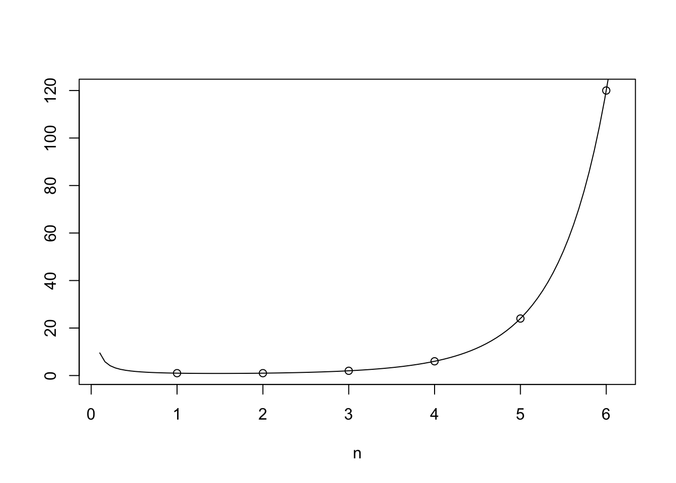
Figure 38.1 shows the gamma function on top of \((n - 1)!\) (for integer values of \(n\)). Notice how the gamma function connects the dots, allowing us to make sense of non-integer factorials, like \(3.5!\).
Therefore, we can replace \((n-1)!\) in Equation 38.1 with \(\Gamma(n)\) and generalize the gamma distribution to non-integer parameters. As a reminder that \(n\) need not be an integer, we will rename this parameter to \(\alpha\).
When the shape parameter \(\alpha\) is not an integer, the gamma distribution does not have a natural interpretation (unlike for integer values of \(\alpha\), where it can be interpreted as the sum of i.i.d. exponentials). Nevertheless, non-integer shape parameters afford us flexibility in modeling.
Next, we calculate formulas for the expected value and variance. Previously, we obtained these formulas for integer shape parameters, by representing the gamma random variable as a sum of i.i.d. exponentials and appealing to linearity of expectation. However, to prove these formulas for general gamma distributions, we have to evaluate an integral.
Of course, we could have also derived the expectation and variance if we knew its moment generating function. The MGF is derived below; Exercise 38.1 asks you to rederive the expectation and variance using Equation 38.5.
The MGF provides quick proofs of the following properties.
Proposition 38.4 is intuitive when both \(\alpha\) and \(\beta\) are integers because then \(X\) is the sum of \(\alpha\) i.i.d. exponentials and \(Y\) is the sum of \(\beta\) i.i.d. exponentials.
- If we scale \(X\) by \(a\), that is equivalent to scaling each exponential by \(a\), which we know from Proposition 22.3 results in an exponential with rate \(\lambda / a\). Therefore, we are simply adding \(\alpha\) i.i.d. exponential random variables with rate \(\lambda / a\), which follows a \(\text{Gamma}(\alpha, \frac{\lambda}{a})\) distribution.
- If we add \(X\) and \(Y\), then together they represent the sum of \(\alpha + \beta\) i.i.d. exponentials, which follows a \(\text{Gamma}(\alpha + \beta, \lambda)\) distribution.
Now that we know the gamma distribution and its properties, we can return to the problem posed at the beginning of this chapter, which was a motivating example for this entire unit.
One of the advantages of calculating the exact bias (which was only possible because we knew the exact distribution of \(\bar X\)) is that it suggests an unbiased estimator of \(\lambda\). Exercise 38.3 asks you to find such an estimator and compare its MSE with the MLE \(\hat\lambda\).
38.2 Maximum Likelihood Estimation
Now that we can model data using the gamma distribution with non-integer values of \(\alpha\), how do we find the best value of \(\alpha\) for a given data set? The answer is maximum likelihood, of course.
The likelihood for a sample of data \(X_1, \dots, X_n\) is \[ L(\alpha, \lambda) = \prod_{i=1}^n \frac{\lambda^\alpha}{\Gamma(\alpha)} X_i^{\alpha - 1} e^{-\lambda X_i}, \] so the log-likelihood is \[ \ell(\alpha, \lambda) = n\alpha \log\lambda - n\log\Gamma(\alpha) + (\alpha - 1) \sum_{i=1}^n \log X_i - \lambda \sum_{i=1}^n X_i.\]
If we know \(\alpha\), then the optimal \(\lambda\) satisfies \[ \frac{\partial\ell}{\partial\lambda} = \frac{n\alpha}{\lambda} - \sum_{i=1}^n X_i = 0, \] so the optimal value of \(\lambda\) (for a given value of \(\alpha\)) is \[ \hat\lambda(\alpha) = \frac{\alpha}{\bar X}. \tag{38.8}\]
Substituting this back into the log-likelihood, we see that the optimal \(\alpha\) must maximize \[ \ell(\alpha, \hat\lambda(\alpha)) = n\alpha \log \frac{\alpha}{\bar X} - n\log\Gamma(\alpha) + (\alpha - 1) \sum_{i=1}^n \log X_i - n\alpha \] or equivalently, \[ J(\alpha) = \frac{1}{n} \ell(\alpha, \hat\lambda(\alpha)) = \alpha \log \frac{\alpha}{\bar X} - \log\Gamma(\alpha) + (\alpha - 1) \frac{1}{n} \sum_{i=1}^n \log X_i - \alpha. \tag{38.9}\]
Solving for the optimal \(\alpha\) by hand is hopeless, not least because there is an \(\alpha\) nested inside a gamma function. However, for any given data set, we can find the optimal \(\alpha\) numerically using Newton’s method.
Example 38.2 (Newton’s method for maximum likelihood)
Isaac Newton (1643-1727)
Newton’s method, first published by Isaac Newton in 1669, is a general method for maximizing (or minimizing) a function \(J(\alpha)\).
We start with a guess for \(\alpha\) and iteratively update the guess as follows: \[ \alpha \leftarrow \alpha - \frac{J'(\alpha)}{J''(\alpha)}. \tag{38.10}\] After several iterations, \(\alpha\) will converge to a (local) maximum or minimum.
To maximize Equation 38.9 using Newton’s method, we will first need to calculate its derivatives.
The first derivative is \[ J'(\alpha) = \log\alpha - \log \bar X - \underbrace{\frac{\Gamma'(\alpha)}{\Gamma(\alpha)}}_{\psi(\alpha)} + \frac{1}{n}\sum_{i=1}^n \log X_i \] and involves the digamma function \(\psi(\alpha) \overset{\text{def}}{=}\frac{\Gamma'(\alpha)}{\Gamma(\alpha)}\), built into many scientific programming libraries and languages, including R.
The second derivative is \[ J''(\alpha) = \frac{1}{\alpha} - \psi'(\alpha), \] which involves the derivative of the digamma function, called the trigamma function.
Now, we implement Newton’s method on the prices data from above in R.
Notice that Newton’s method converges after only about 5 or 6 iterations. Try different starting guesses for \(\alpha\). No matter where you start, Newton’s method should converge to the same estimate.
Now that we have the optimal value of \(\alpha\), we can plug it into Equation 38.8 to obtain the corresponding value of \(\lambda\). Finally, we plot the fitted gamma distribution on top of the data.
If the fit of this curve to the data is disappointing, the gamma distribution is not to blame! This is merely the member of the gamma family that fits this data the best. The fact that it does not fit the data particularly well suggests that we may want to look beyond the gamma distribution for a model.
38.3 Chi-Square Distribution
The gamma distribution with non-integer shape parameter \(\alpha\) also arises in the guise of the chi-square, or \(\chi^2\), distribution, an important distribution in statistics, which will figure prominently in Chapter 45.
Let \(Z_1, \dots, Z_k\) be i.i.d. standard normal. The random variable \[S_k = Z_1^2 + \dots + Z_k^2\] is said to follow a \(\chi^2_k\) distribution. But the \(\chi^2_k\) distribution is not new; it is merely a special case of the gamma distribution!
38.4 Exercises
Exercise 38.1 (Deriving the gamma expectation and variance using MGFs) Rederive the expectation and variance of the gamma distribution (Proposition 38.2) using the MGF of the gamma distribution (Equation 38.5).
Exercise 38.2 (Moments of the gamma distribution) Let \(X \sim \text{Gamma}(\alpha, \lambda)\) and \(k\) be a positive integer. Use the moment generating function to show that \[ \text{E}\!\left[ X^k \right] = C_k \frac{\Gamma(\alpha+k)}{\Gamma(\alpha)} \] for some constant \(C_k\) (that depends on \(k\)). What is \(C_k\)?
Exercise 38.3 (Comparing estimators of the exponential rate parameter) In Example 38.1, we determined the bias of the MLE \(\hat\lambda\) of the rate parameter \(\lambda\) from i.i.d. observations \(X_1, \dots, X_n \sim \text{Exponential}(\lambda)\). We will assume \(n > 2\).
- Use the results to propose an unbiased estimator \(\hat\lambda_{\text{unbiased}}\) of \(\lambda\).
- Calculate the MSE of \(\hat\lambda\).
- Calculate the MSE of \(\hat\lambda_{\text{unbiased}}\).
- Which estimator is better?
(Hint: You should be able to calculate \(\text{E}\!\left[ \frac{1}{\bar X^2} \right]\) in a similar way to Example 38.1.)
Exercise 38.4 (Moments of the exponential distribution) Let \(X \sim \text{Exponential}(\lambda)\). Show that \[ \text{E}\!\left[ X^k \right] = \frac{k!}{\lambda^k} \] for any positive integer \(k\).
Exercise 38.5 (Modeling rainfall using the gamma distribution) The total rain water collected in the Crystal Springs Reservoir in a year is gamma distributed with mean \(1000\) gallons and standard deviation \(300\) gallons. Assuming rain is independent year to year, what is the probability that
- the total rainwater collected by the reservoir in two years is less than \(2500\) gallons?
- more than average collection of rain water happens in at least three of the next five years?
Exercise 38.6 (Relationship between the gamma and Poisson distributions) Let \(\alpha\) be a positive integer.
- Show that \[ \int_x^\infty \frac{1}{\Gamma(\alpha)} z^{\alpha - 1} e^{-z} \, dz = \sum_{y=0}^{\alpha-1} \frac{x^y e^{-x}}{y!}. \]
- If \(X \sim \text{Gamma}(\alpha,\lambda)\), show that \[ P(X \leq x) = P(Y \geq \alpha), \] where \(Y \sim \text{Poisson}(\lambda x)\).
Exercise 38.7 (Why the Rayleigh distribution is useful for modeling wind speeds) In Exercise 30.3, you modeled wind speeds using the Rayleigh distribution. Here, we will give a physical motivation for why the Rayleigh distribution is reasonable for modeling wind speeds.
Let \(X\) be the east-west wind velocity, where a positive velocity indicates that the wind is blowing east. Let \(Y\) be the north-south wind velocity. Then, the wind speed is the magnitude of the velocity vector: \[ W = \sqrt{X^2 + Y^2}. \] Show that if \(X\) and \(Y\) are independent \(\text{Normal}(0, \sigma^2)\), then \(W\) follows a Rayleigh distribution (Equation 30.12).
Hint: First, determine the distribution of \(W^2\), which is related to the distributions in this chapter.
Exercise 38.8 (Estimating the precision) Let \(X_1, \dots, X_n\) be i.i.d. \(\text{Normal}(0, \sigma^2)\). Consider estimating the precision \(\phi = \frac{1}{\sigma^2}\).
- What is the MLE of \(\phi\)?
- For what value of \(\alpha\) is the estimator \(\frac{\alpha}{\sum_{i=1}^n X_i^2}\) unbiased for \(\phi\)?