5 Conditional Probability

You walk by a roulette wheel at a casino (Figure 1.5) and stop to watch. The ball lands in a red pocket on $9$ spins in a row. You wonder if you should enter the action at this point, betting on black. After all, the probability of $10$ reds in a row is very small, only \[ P(\text{all 10 spins are red}) = \frac{18^{10}}{38^{10}} \approx .00057. \tag{5.1}\] In particular, it is much lower than the probability of $1$ black and $9$ reds in the $10$ spins: \[ P(\text{1 black, 9 reds in 10 spins}) = \frac{{10 \choose 1} 18^{1}18^{9}}{38^{10}} \approx .0057. \]

Where is the flaw in this argument? The calculations are correct; the problem is that these probabilities are not relevant to the decision you want to make. The $9$ reds have already happened, so there is no reason to calculate their probability. Instead, we should be using this information to update the probability that that the 10th spin is red. We write this updated probability as \[ P(\text{10th spin is red}\ |\ \text{first 9 spins are red}), \tag{5.2}\] called a conditional probability. This is more relevant to your decision than the joint probability (Equation 5.1).

In this chapter, we will discuss how to calculate conditional probabilities, as a way to update probabilities in light of new information. By the end of this chapter, we will be able to calculate Equation 5.2 and answer the question of whether you should bet on black.

5.1 Definition of Conditional Probability

To motivate the definition of conditional probability, we recall the Secret Santa example (Example 1.7). Four friends write their names on slips of paper, put the slips in a box, shake the box, and each draw a name. Now suppose that after drawing the first slip, the first friend announces that she did not draw her own name. How does this information change the probability that the second friend draws his own name?

Representing each friend with a number from 1 to 4 (as we did in Example 1.7), we recall the $24$ equally likely outcomes in our sample space. Bolded entries are the outcomes where the second friend draws his own name:

1. 1234	7. 2134	13. 3124	19. 4123
2. 1243	8. 2143	14. 3142	20. 4132
3. 1324	9. 2314	15. 3214	21. 4213
4. 1342	10. 2341	16. 3241	22. 4231
5. 1423	11. 2413	17. 3412	23. 4312
6. 1432	12. 2431	18. 3421	24. 4321

We see that, initially, the probability of the second friend drawing his own name is $6/24 = .25$, which makes sense because of symmetry.

However, upon learning that the first friend did not draw her own name, we can remove all outcomes where she does, leaving us with a reduced, but still equally likely, set of possible outcomes:

1. 1234	7. 2134	13. 3124	19. 4123
2. 1243	8. 2143	14. 3142	20. 4132
~~3. 1324~~	9. 2314	15. 3214	21. 4213
~~4. 1342~~	10. 2341	16. 3241	22. 4231
~~5. 1423~~	11. 2413	17. 3412	23. 4312
~~6. 1432~~	12. 2431	18. 3421	24. 4321

The second friend only draws his own name in $4$ of the remaining outcomes, so the probability that he draws his own name has decreased to $4/18 \approx .222$. This result makes sense: if the first friend did not draw her own name, then she is more likely to have drawn the second friend’s name. This should reduce the chance that the second friend draws his own name.

This is an example of a conditional probability. The conditional probability $P(A|B)$ (read as “probability of $A$ given $B$”) is the probability of $A$ happening if we know that $B$ has happened. As we saw above, knowing that $B$ has happened gives important partial information about the experiment’s outcome (i.e., we know it must be in $B$), forcing us to update our assessment of how likely $A$ is to happen.

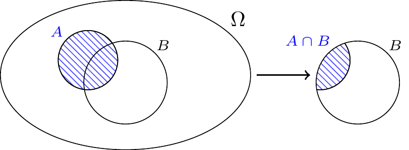
Before giving a formal definition of conditional probability, we first motivate it visually in Figure 5.1. This diagram illustrates how the event $A$ occupies a portion of the sample space $\Omega$ and the restricted space $B$.

Figure 5.1: Illustration of the proportion of $\Omega$ taken up by $A$, compared with the proportion of $B$ taken up by $A$ (specifically, the part of $A$ that is in $B$).

Like before, the probability $P(A)$ is the proportion of the sample space $\Omega$ taken up by $A$ (shaded in blue on the left). However, if we know that $B$ has happened, then we should restrict to outcomes in $B$. The most natural definition of the conditional probability $P(A|B)$ is then the proportion of the restricted space $B$ taken up by $A$ (specifically, the part of $A$ that is in $B$).

Definition 5.1 formalizes this idea.

Definition 5.1 (Conditional probability) For two events $A$ and $B$ with $P(B) > 0$, the conditional probability of $A$ given $B$ is \[ P(A | B) \overset{\text{def}}{=}\frac{ P(A \cap B)}{P(B)} \tag{5.3}\]

Events with zero probability

The definition doesn’t apply when $B$ has zero probability (i.e., $P(B) = 0$) because it would require dividing by $0$. Intuitively, probability zero events never happen, so there would be no need to define probabilities conditional on them happening.

The frequentist interpretation of the conditional probability $P(A|B)$ is straightforward: it is the proportion of times that $A$ happens as the experiment is repeated over and over, ignoring the experiments where $B$ did not happen. At the end of this chapter, we will discuss why Definition 5.1 is the right definition for capturing this interpretation.

Our first example uses Definition 5.1 to formally answer Secret Santa.

Example 5.1 (Conditional Secret Santa) If we know that the first friend did not draw her own name in Secret Santa, what is the probability that the second friend draws his own name?

The sample space $\Omega$, previously enumerated in Table 1.1, consists of $24$ equally likely outcomes. Letting $A_i$ be the event that the $i$th friend draws their own name, the probability of interest is $P(A_2| A_1^c)$. By Definition 5.1, this is

\[ \begin{align*} P(A_2 | A_1^c) &= \frac{P(A_2 \cap A_1^c)}{P(A_1^c)} & \text{(definition of conditional probability)}\\ &= \frac{\frac{4}{24}}{\frac{18}{24}} & \text{(counting outcomes)} \\ &= \frac{4}{18} \end{align*} \] Like earlier, we find that $P(A_2| A_1^c) = 2/9 \approx 0.22.$

In some cases, conditional probabilities can be quite counterintuitive. To ensure that we correctly handle cases like our next example, it is imperative that we carefully apply Definition 5.1 when we want to compute conditional probabilities, and not just rely on intuition.

Example 5.2 (The boy-girl paradox) Suppose we meet a family at a dinner party and learn in conversation that they have two children. Consider the following two scenarios:

Scenario One: We learn that at least one of the children is a girl (e.g., “We have two children. One of them is on the women’s swim team.”)
Scenario Two: We learn that the eldest child is a girl (e.g., “We have two children. Our eldest is on women’s swim team.”)

In each scenario, what’s the probability that both of the children are girls?

Upon a first read, it may feel that the two scenarios are the same; in both of them we learn that one child is a girl and nothing about the other. In actuality however, the two scenarios lead to different answers!

Marking the gender of the older child first and the younger child second, there are four possible equally likely outcomes in our sample space $\Omega = \{BB, BG, GB, GG\}$. We can apply Definition 5.1 to compute the relevant probability in each case.

Solution to Scenario One: To find the solution in Scenario One, we directly apply Definition 5.1:

\[ \begin{align*} P( 2 \text{ girls}| \geq 1 \text{ girl}) &= \frac{P( 2 \text{ girls and } \geq 1 \text{ girl}) }{P(\geq 1 \text{ girl}) } & \text{(definition of conditional probability)}\\ &= \frac{P(2 \text{ girls}) }{P(\geq 1 \text{ girl})} & \text{(\{} 2 \text{ girls\}} \cap \text{\{} \geq 1 \text{ girl\}} = \text{\{} 2 \text{ girls\})} \\ &= \frac{P( \{GG \}) }{P(\{GG, GB, BG \} )} & \text{(write out outcomes in each event)}\\ &= \frac{1}{3}. & \text{(count equally likely outcomes)} \end{align*} \]

Solution to Scenario Two: We can follow the same reasoning to find the solution in Scenario Two:

\[\begin{align*} P( 2 \text{ girls}| \text{eldest girl}) &= \frac{P( 2 \text{ girls and eldest is girl}) }{P(\text{eldest is girl}) } & \text{(definition of conditional probability)}\\ &= \frac{P(2 \text{ girls}) }{P(\text{eldest is girl})} & \text{(\{} 2 \text{ girls\}} \cap \text{\{eldest is girl\}} = \text{\{} 2 \text{ girls\})} \\ &= \frac{P( \{GG \}) }{P(\{GG, GB\} )} & \text{(write out outcomes in each event)}\\ &= \frac{1}{2}. & \text{(count equally likely outcomes)} \end{align*}\]

As we suggested, the probabilities aren’t the same. In the first scenario, we learn that at least one child is a girl, leaving two ways for the couple to also have a boy ($BG$ and $GB$). In the second scenario we learn that a specific child (the eldest) is a girl, leaving just one way for the couple to also have a boy ($GB$).

Now we consider a perhaps even more counter-intuitive third scenario.

Scenario Three: We meet a random one of the two children and learn that they are a girl (e.g., “One of our children happens to be walking over right now. She’s on the women’s swim team.”)

Since we meet a random child (not a specific one, like the eldest), this may feel more like Scenario One, where all we learn is that at least one child is a girl. It turns out to be more like Scenario Two, however, because by meeting a child, we still unambiguously nail down the gender of one of the children (albeit, a random one). This is something we were unable to do in Scenario One.

Solution to Scenario Three: In Scenario Three, there’s additional randomness due to the fact that we randomly meet one of the children. To properly analyze this scenario, we need to augment our sample space to capture this randomness: \[ \Omega = \{\underline{B}B, \underline{B}G, \underline{G}B, \underline{G}G, B\underline{B}, B\underline{G}, G\underline{B}, G\underline{G} \} . \] We still specify the gender of the older child first and the younger one second, but now the underlined letter indicates which child we meet. We will assume that these outcomes are equally likely—that is, regardless of their genders, it is a coin toss whether we meet the youngest or eldest child). Now, we can calculate the probability.

\[\begin{align*} P(2 \text{ girls}| \text{meet girl}) &= \frac{P(2 \text{ girls and meet girl}) }{P(\text{meet girl})} & \text{(definition of conditional probability)} \\ &=\frac{P( \{\underline{G}G, G\underline{G} \}) }{P(\{\underline{G}B, \underline{G}G, B\underline{G}, G\underline{G} \} )} & \text{(write out outcomes in each event)}\\ &= \frac{1}{2}. & (\text{count equally likely outcomes}) \end{align*}\]

5.2 The Multiplication Rule

We can also combine the conditional probabilities to obtain the probability that multiple events happen simultaneously. To build some intuition as to why, we begin with a simple example. Say we draw the two cards from the top of a shuffled deck of $52$ playing cards (see Figure 1.6). What is the probability that both cards are spades?

Because there are $13$ spades in the deck, the first card should be a spade $\frac{13}{52}$ of the time. Given that the first card is a spade, there are $12$ spades remaining in a deck of $51$ cards, so the second card will also be a spade $\frac{12}{51}$ of the time. For both cards to be spades, both these events need to happen. This should happen $12/51$ of $13/52$ the time, or, in other words, $\frac{13}{52} \cdot \frac{12}{51}$ of the time.

This is the idea behind the multiplication rule, which really is just a restatement of the definition of conditional probability (Definition 5.1).

Corollary 5.1 (Multiplication rule for two events) If $A$ and $B$ are two events with $P(A) > 0$ and $P(B) > 0$, then \[ P(A \cap B) = P(B) P(A | B) = P(A) P(B | A). \tag{5.4}\]

Probability zero events

If either $P(A) = 0$ or $P(B) = 0$, then we can immediately conclude that $P(A \cap B) = 0$ also. This is because $P(A \cap B) \leq P(A)$ and $P(A \cap B) \leq P(B)$ by the subset rule (Proposition 4.3).

Proof

The definition of conditional probability (Definition 5.1) says that \[P(A|B) = \frac{P(A \cap B)}{P(B)}\] Multiplying both sides by $P(B)$ we get that $P(B)P(A|B) = P(A\cap B)$.

Applying the same argument to $P(B|A)$ gives that $P(A) P(B |A) = P(A \cap B)$.

The multiplication rule is useful when the conditional probability $P(A | B)$ is easy to determine, but the joint probability $P(A \cap B)$ is not. The next example provides such a scenario.

Example 5.3 (NBA Draft Lottery) The National Basketball Association (NBA) conducts a draft each year where teams select new talent. Since there are a few superstars each year, the first few draft picks are highly coveted. The order for the first three picks is determined by a lottery that is weighted so that the worst teams have the best chances of getting these picks.

Between 1990 and 1994, the lottery worked as follows: each of the 11 teams that did not make the playoffs the previous season would have a certain number of ping-pong balls with their names on them. The team with the worst record would have 11 balls, the team with the second-worst record would have 10 balls, and so on, down to the team with the best record, which would only have 1 ball—for a total of 66 balls. First, a ball was drawn to determine the team that gets the first pick. All of this team’s balls were removed, and another ball was drawn to determine the team that gets the second pick. All of this team’s balls were removed as well, and a third ball was drawn to determine the team that gets the third pick.

The 1992 NBA draft had one of the most talented pools ever. The 11 teams that were eligible for the top three picks, based on their win-loss record in the 1991-92 season, were:

Houston Rockets (1 ball)
Atlanta Hawks (2 balls)
Philadelphia 76ers (3 balls)
Charlotte Hornets (4 balls)
Milwaukee Bucks (5 balls)
Sacramento Kings (6 balls)
Washington Bullets (7 balls)
Denver Nuggets (8 balls)
Dallas Mavericks (9 balls)
Orlando Magic (10 balls)
Minnesota Timberwolves (11 balls)

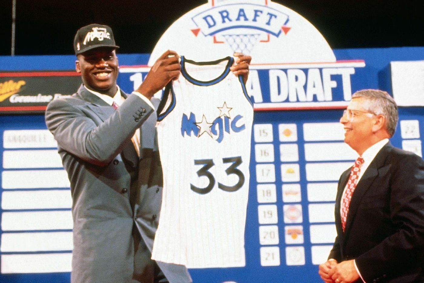
Figure 5.2: #1 1992 draft pick Shaquille O’Neal

The teams that actually received the top 2 draft picks were the Orlando Magic (who selected Shaquille O’Neal) and Charlotte Hornets (who selected Alonzo Mourning). What was the probability of this? In other words, we want to calculate the joint probability \[ P(\{\text{Magic get 1st pick}\} \cap \{\text{Hornets get 2nd pick}\}). \]

It is not straightforward to describe a sample space of equally likely outcomes for the first two picks in this weighted lottery. (If you don’t see why, try it!) The problem is that the number of balls remaining for the second pick depends on which team got the first pick.

However, it is easy to reason about the conditional probabilities. For example, \[ P(\text{Hornets get 2nd pick}\ |\ \text{Magic get 1st pick}) = \frac{4}{56} \] because if the Magic get the first pick, then there are $66 - 10 = 56$ balls remaining, of which $4$ belong to the Hornets.

Now, we can calculate the joint probability from the multiplication rule (Corollary 5.1). \[ \begin{align} P(\{\text{Magic get 1st pick}\} &\cap \{\text{Hornets get 2nd pick}\}) \\ &= P(\text{Magic get 1st pick}) P(\text{Hornets get 2nd pick}\ |\ \text{Magic get 1st pick}) \\ &= \frac{10}{66} \cdot \frac{4}{56} \\ &\approx .01. \end{align} \]

What is the probability that the first card on top of a shuffled deck of $52$ playing cards is a spade? It is not hard to see that it is $13/52$ by simply counting the spades. But what about the probability that the second card is a spade? The conditional probabilities are easy to calculate, by restricting the sample space to the $51$ remaining cards after the first card is removed:

$P(\text{2nd card spade}\ |\ \text{1st card spade}) = \frac{12}{51}$
$P(\text{2nd card spade}\ |\ \text{1st card not spade}) = \frac{13}{51}$

But what about the unconditional probability that the second card is a spade? By symmetry, the answer must be $13/52$. In a well-shuffled deck, there is nothing special about the 2nd card or the 35th card. If we have no other information, every card is equally likely to be any one of the 52 cards.

If you are not convinced by the symmetry argument, the next example, based on the multiplication rule, may help.

Example 5.4 (Selecting cards and probability trees) Suppose we draw two cards from the top of a shuffled deck of $52$ playing cards. What is the probability that both cards are spades? What about the probability that the first card is not a spade but the second card is?

Let $S_1$ be the event that the first card is a spade and $S_2$ be the event that the second card is a spade. As we argued above,

$P(S_2 | S_1) = \frac{12}{51}$
$P(S_2 | S_1^c) = \frac{13}{51}$

However, it is not immediately obvious what $P(S_1 \cap S_2)$ is.

One way to visualize these conditional probabilities and the multiplication rule is to draw a probability tree.

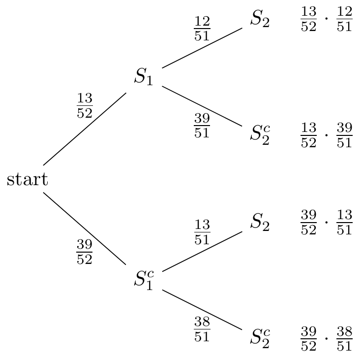
Each branch’s label shows the conditional probability of the event, given all the preceding events. For example:

Path through $S_1$ and $S_2$: The path through $S_1$ and $S_2$ tells us that $P(S_1) = \frac{13}{52}$ and $P(S_2 | S_1) = \frac{12}{51}$.
Path through $S_1^c$ and $S_2$: The path through $S_1^c$ and $S_2$ tells us that $P(S_1^c) = \frac{39}{52}$ and $P(S_2|S_1^c) = \frac{13}{51}$.

At the end of each path, we write the product of all the probabilities along the path. The multiplication rule (Corollary 5.1) tells us that this final number is the joint probability of all of those events. For example:

Drawing two spades: To find the probability of drawing two spades, we can follow the path through $S_1$ and $S_2$ to find that $P(S_1 \cap S_2) = P(S_1)P(S_2|S_1) = \frac{13}{52} \cdot \frac{12}{51}$ at the end.
Drawing a non-spade and then a spade: Following the path through $S_1^c$ and $S_2$ we see that the probability that both the cards are not spades is $P(S_1^c \cap S_2) = P(S_1^c) P(S_2| S^c_1) = \frac{39}{52} \cdot \frac{13}{51}$.

These are the two (mutually exclusive) ways that the second card can be a spade. Therefore, we can calculate the probability that the second card is a spade by adding these two probabilities together: \[ P(S_2) = \frac{13}{52} \cdot \frac{12}{51} + \frac{39}{52} \cdot \frac{13}{51} = \frac{13}{52}, \] which agrees with the symmetry argument we made earlier.

Probability trees quickly become unwieldy with a larger number of events. Still, they are a popular way of representing conditional probabilities and can be helpful for simple problems.

The multiplication rule realizes its full potential when generalized to more than two events. Before introducing this generalization, we first introduce some shorthand notation.

When working with many events $A_1, \dots, A_n$, using $P(A_1 \cap \dots \cap A_n)$ to denote the probability of all the events happening becomes cumbersome. Instead, we will adopt the shorthand notation

\[ P(A_1, \dots, A_n) \overset{\text{def}}{=}P(A_1 \cap \dots \cap A_n), \tag{5.5}\]

where commas inside a probability $P(\dots)$ are read as “and”. For example,

$P(A_1, A_2, A_3)$ is the probability of “$A_1 \text{ and } A_2 \text{ and } A_3$” happening.
$P(A| B_1, \dots, B_n)$ is the probability of $A$ happening, given that “$B_1 \text{ and } B_2 \text{ and } \dots \text{ and } B_n$” have all happened.

With this new notation, we can state the general multiplication rule.

Theorem 5.1 (Multiplication rule) For events $A_1, \dots, A_n$ with positive probability, \[ P(A_1, A_2, \dots A_n) = P(A_1) P(A_2 | A_1) P(A_3 | A_1, A_2) \dots P(A_n| A_1, \dots A_{n-1}) \tag{5.6}\]

Proof

The multiplication rule is formally proved by mathematical induction. Rather than give a formal proof, we’ll provide a more illustrative argument. Looking at the right-hand side of Equation 5.6, we have \[ \textcolor{blue}{P(A_1) P(A_2 | A_1)} P(A_3 | A_1, A_2) \dots P(A_n| A_1, \dots, A_{n-1}) \] The multiplication rule for two events (Corollary 5.1) tells us that the highlighted part can be written as
\[ P(A_1) P(A_2| A_1) = P(A_1, A_2). \] Substituting this back in, the right hand side is now \[ \textcolor{blue}{P(A_1, A_2) P(A_3 | A_1, A_2)} \dots P(A_n| A_1, \dots, A_{n-1}) \] Another application of the multiplication rule for two events (the first event is $A_3$ and the second is $A_1 \cap A_2$) tells us that the new highlighted part can be written as

\[ P(A_1, A_2) P(A_3| A_1, A_2) = P(A_1, A_2, A_3). \]

Substituting this back in, the right hand side is now \[ \textcolor{blue}{P(A_1, A_2, A_3) P(A_4 | A_1, A_2, A_3)} \dots P(A_n| A_1, \dots, A_{n-1}) \]

Continuing this argument, all of these probabilities will eventually combine into $P(A_1, \dots, A_n)$.

Ordering is arbitrary

Since the ordering of the events was arbitrary, we can apply the multiplication rule to any reordering of them (as was the case in Corollary 5.1). For example, it’s both true that \[ P(A_1 , A_2, A_3) = P(A_3) P(A_2 | A_3) P(A_1|A_2, A_3), \] and that \[ P(A_1 , A_2, A_3) = P(A_2) P(A_1 | A_2) P(A_3|A_1, A_2). \] Because there are $n!$ ways to order the events (by Corollary 2.1), the multiplication rule is actually $n!$ theorems for the price of one!

In many settings, the multiplication rule enables us to easily compute the joint probability that many events happen simultaneously.

Example 5.5 (Probability of a flush) Suppose we are playing five-card draw poker (see the relevant part of Chapter 2 for a review of poker), and are dealt our hand from the top of a shuffled deck. What is the probability that we get a flush (five cards of the same suit)?

The event of getting a flush can be written as the disjoint union of getting a flush of spades, a flush of clubs, a flush of diamonds, or a flush of hearts. Therefore, Axiom 3 (see Definition 3.1) tells us that

\[ P(\text{flush})= P(\spadesuit \text{ flush}) + P(\clubsuit \text{ flush}) + P(\diamondsuit \text{ flush}) + P(\heartsuit \text{ flush}). \]

Let’s focus on computing $P(\spadesuit \text{ flush})$, i.e., the probablity that we draw all spades. The remaining probabilities should be equal by symmetry (there is nothing special about spades compared to the other suits). Letting $S_i$ be the event that the $i$th card we draw is a spade, we can apply the multiplication rule (Theorem 5.1): \[\begin{align*} &P(\spadesuit \text{ flush}) &\\ &= P(S_1) P(S_2 | S_1) \dots P(S_5| S_4, S_3, S_2, S_1) & \text{(multiplication rule)}\\ &= \frac{13}{52} \cdot \frac{12}{51} \cdot \frac{11}{50} \cdot \frac{10}{49} \cdot \frac{9}{48} & \text{(equally likely to get any remaining card)} \end{align*}\]

Indeed, the same argument applies to the other suits as well, implying that

\[ P(\text{flush}) = 4 \times \frac{13 \times 12 \times 11 \times 10 \times 9}{52 \times 51 \times 50 \times 49 \times 48} \approx 0.002. \]

Note that drawing a probability tree for this problem would have required drawing $2^5 = 32$ different paths!

In our next example, we explore how the multiplication rule naturally appears in large language models, which are used by AI systems to generate text.

Example 5.6 (Decoding a large language model) How does a large language model (LLM) learn to output coherent phrases like $\text{``beware of the dog''}$, rather than jumbled phrases like $\text{``dog the beware of''}$? The answer turns out to be intimately related to conditional probabilities and the multiplication rule.

LLMs generate one word at a time, given all of the previous words. Therefore, an LLM needs to know the probability of seeing a particular word next, given a sequence of words. For example, an LLM may tell us that:

\[ \begin{array}{l} P(\text{``aardvark'' next} | \text{``beware of the'' so far}) = .0002 \\ \hspace{4cm} \vdots \\ P(\text{``dog'' next} | \text{``beware of the'' so far}) = .1 \\ \hspace{4cm} \vdots \\ P(\text{``zyzzyva'' next} | \text{``beware of the'' so far}) = .000006 \\ \end{array} \]

LLMs learn these probabilities by analyzing patterns across huge amounts of text, known as the training data. In our example, our hypothetical LLM has learned that $\text{``dog''}$ follows $\text{``beware of the"}$ about 10% of the time.

So how can we generate text from an LLM? One reasonable idea is to start with a word, either randomly or provided by a user, such as $\text{``beware''}$. Then we tack on the most likely next word, given that the first word was , such as $\text{``beware of''}$. This process continues until the most likely next “word” is a ${\tt STOP}$ token, resulting in a complete phrase such as $\text{``beware of the dog''}$. According to the multiplication rule (Corollary 5.1),

\[ \begin{align} &P(\text{``beware of the dog''}) \\ &= P(\text{``beware'''}) \cdot P(\text{``of" next} | \text{``beware" so far} ) \\ &\quad \cdot P(\text{``the" next} | \text{ ``beware of " so far} ) \cdot P(\text{``dog" next} | \text{ ``beware of the " so far} ) \\ &\quad \cdot P({\tt STOP} | \text{ ``beware of the dog" so far} ) \end{align} \tag{5.7}\]

Therefore, by picking words with high conditional probabilities of appearing next (the right-hand side of Equation 5.7), we ensure that the outputted phrase has a high overall probability (the left-hand side of Equation 5.7). For example, if our LLM encodes probabilities

\[ \begin{array}{ll} P(\text{``beware''}) = 0.001, & P(\text{``dog''}) = 0.0005, \\ P(\text{``of'' next} | \text{``beware'' so far}) = 0.65, & P(\text{``the'' next} | \text{``dog'' so far}) = 0.0008, \\ P(\text{``the'' next} | \text{``beware of'' so far}) = 0.32, & P(\text{``beware'' next} | \text{``dog the'' so far}) = 0.00007, \\ P(\text{``dog'' next} | \text{``beware of the'' so far}) = 0.9, & P(\text{``of'' next} | \text{``dog the beware'' so far}) = 0.004, \\ P({\tt STOP} | \text{``beware of the dog'' so far}) = 0.1, & P({\tt STOP} | \text{``dog the beware of'' so far}) = 0.0001, \\ \end{array} \]

then the multiplication rule tells us that

\[ \begin{array}{l} P(\text{``beware of the dog''}) = 0.001 \cdot 0.65 \cdot 0.32 \cdot 0.9 \cdot 0.1 \approx 0.00002 \\ P(\text{``dog the beware of''}) = 0.0005 \cdot 0.0008 \cdot 0.00007 \cdot 0.004 \cdot 0.0001 \approx 0.0000000000000001. \\ \end{array} \] By generating one word at a time using conditional probabilities, the LLM generates phrases that have a higher overall probability—at least based on the training data. As long as the model was trained on coherent text, we should expect these outputted phrases to be coherent as well.

Randomized decoding

If we actually had an LLM pick the highest probability word given the previous words, it would output the same phrase every time it started with a particular word. Instead, we may randomly sample the next word according to the probabilities of the model. Words with higher conditional probabilities of being next are more likely to be sampled, and this way we can get the LLM to output a variety of phrases that are all coherent.

Tokens versus words

We described LLMs as generating words for simplicity. However, in practice, most LLMs generate tokens instead of words. Tokens may be words, but they are usually shorter fragments that may include spaces and punctuation, such as “bew” or “ar” or “e o”.

5.3 Conditional Probability Functions

A probability function $P$ allocates a total probability of $1$ among all outcomes in the sample space $\Omega$. Conditioning on an event $B$ reallocates this probability so that only outcomes in $B$ are considered. In this new allocation, outcomes outside of $B$ receive zero probability, while the probabilities of outcomes in $B$ are rescaled proportionally so that the total probability is $1$.

Proposition 5.1 formalizes this idea. In particular, it says that conditioning on an event is equivalent to defining a new probability function.

Proposition 5.1 (Conditional probabilities are probability functions) Let $P$ be a probability function. For any event $B$ with positive probability $P(B) > 0$, consider the function $\widetilde P$ defined by \[ \widetilde{P}(A) \overset{\text{def}}{=}P(A | B). \]

Then $\widetilde P$ is also a probability function in that it satisfies Kolmogorov’s axioms (Definition 3.1).

Proof

To show that $\widetilde P$ is a valid probability function, we check that it satisfies each of the axioms of Definition 3.1:

Axiom 1: Because $P$ satisfies Axiom 1, we know that $P(A \cap B) \geq 0$. Therefore, \[ \widetilde{P}(A) = P(A|B) = \frac{P(A \cap B)}{P(B)} \geq 0. \]
Axiom 2: Because $B \subset \Omega$ we know that $B \cap \Omega = B$ (see Figure 4.3). Therefore \[ \widetilde{P}(\Omega) = P(\Omega | B) = \frac{P(\Omega \cap B)}{P(B)} = \frac{P(B)}{P(B)} = 1.\]
Axiom 3: Let $A_1, A_2, \dots$ be disjoint sets. Because $A_i \cap B \subseteq A_i$, the countable collection of sets $A_1 \cap B, A_2 \cap B, \dots$ must also be disjoint. Therefore, \[ \begin{align} \widetilde{P}\left( \bigcup_{i=1}^{\infty} A_i \right) &= P\left(\bigcup_{i=1}^{\infty} A_i \bigg| B \right) \\ &= \frac{P\left( \left(\bigcup_{i=1}^{\infty} A_i \right) \cap B \right)}{P(B)} & \text{(definition of conditional probability)}\\ &= \frac{P( \bigcup_{i=1}^{\infty} (A_i \cap B) )}{P(B)} & \text{(distributive property)}\\ &= \frac{\sum_{i=1}^{\infty} P(A_i \cap B)}{P(B)} & \text{($P$ satisfies Axiom 3)}\\ &= \sum_{i=1}^{\infty} \frac{P(A_i \cap B)}{P(B)} & \text{(distribute)}\\ &= \sum_{i=1}^{\infty} P(A_i |B) & \text{(definition of conditional probability)} \\ &= \sum_{i=1}^{\infty} \widetilde{P}(A_i). \end{align} \]

The most important consequence of Proposition 5.1 is that conditional probabilities automatically inherit all of the properties of probability, such as those presented in Chapter 4. We know immediately, for example, that all conditional probabilities also must be between zero and one (see Proposition 4.2). This provides an alternative way to analyze the Linda problem from Example 4.2.

Example 5.7 (The Linda problem revisited) Recall the Linda problem (Example 4.2) from Chapter 4, which concerns a woman named Linda described below:

Linda is 31 years old, single, outspoken, and very bright. She majored in philosophy. As a student, she was deeply concerned with issues of discrimination and social justice, and also participated in anti-nuclear demonstrations.

The Linda problem asks which of the following is more probable:

Linda is a bank teller.
Linda is a bank teller and is active in the feminist movement.

Using the multiplication rule (Theorem 5.1) we see that \[ \begin{align} &P( \text{bank teller and feminist}) & \\ &= P(\text{bank teller}) P(\text{feminist} |\text{bank teller} ) & \text{(multiplication rule)} \\ &\leq P(\text{bank teller}). & \text{(probabilities are between zero and one)} \end{align} \]

We can also analyze a conditional version of the Linda problem, which is perhaps even more counterintuitive than the original problem.

Example 5.8 (A conditional Linda problem) Consider the Linda problem (1), but suppose you learn that all of Linda’s close friends are active in the feminist movement. Given this new information, which of the following is more probable now?

Linda is a bank teller.
Linda is a bank teller and is active in the feminist movement.

With the new information that all of Linda’s close friends are active in the feminist movement, it may now seem possible that the second scenario is more likely. But the event \[ \{ \text{bank teller} \} \cap \{ \text{feminist} \} \] is still a subset of the event \[ \{ \text{bank teller} \}. \] The fact that conditional probability functions are probability functions (Proposition 5.1) enables us to apply the subset rule (Proposition 4.3) to the conditional probability function $\widetilde{P} \overset{\text{def}}{=}P(\cdot | \text{friends are feminists})$ and see that

\[ P(\text{bank teller and feminist} | \text{friends are feminists}) \leq P(\text{bank teller}| \text{friends are feminists}). \]

That is, even given that all of Linda’s friends are active in the feminist movement, the first scenario is still more probable than the second.

Since $\widetilde{P}$ is a probability function, we can further condition on another set $C$ to obtain yet another probability function: \[ \widetilde{\widetilde P}(A) \overset{\text{def}}{=}\widetilde{P}(A | C). \] This corresponds to updating our probabilities twice: first in light of $B$, then in light of $C$. The next result shows that this is equivalent to updating our probabilities based on all the evidence at once, both $B$ and $C$.

Proposition 5.2 (Sequential updating) Let $P$ be a probability function, and let $B$ and $C$ be events such that $P(B \cap C) > 0$.

Now, define the conditional probability functions:

$\widetilde{P}(A) \overset{\text{def}}{=}P(A | B)$
$\widetilde{\widetilde P}(A) \overset{\text{def}}{=}\widetilde{P}(A | C)$.

(Note that these conditional probability functions are both valid, since $P(B) \geq P(B \cap C) > 0$ and $\widetilde P(C) = P(C | B) = \frac{P(B \cap C)}{P(B)} > 0$.)

This sequential updating is equivalent to directly conditioning on $B \cap C$: \[ \widetilde{\widetilde P}(A) = P(A | B, C). \]

Proof

\[ \begin{align} \widetilde{P}( A | C) &= \frac{\widetilde{P}(A, C)}{\widetilde{P}(C)} & \text{(definition of conditional probability)}\\ &= \frac{P(A, C | B)}{P(C | B)} & \text{(definition of conditional probability)}\\ &= \frac{\frac{P(A, B, C)}{P(B)}}{\frac{P(B, C)}{P(B)}} & \text{(definition of $\widetilde{P}$)} \\ &= \frac{P(A, B, C)}{P(B, C)} & \text{(canceling $P(B)$)} \\ &= P(A | B, C) & \text{(definition of conditional probability)} \end{align} \]

Proposition 5.1 and Proposition 5.2 reassure us that conditional probabilities behave like probabilities in all the ways we expect. This makes sense because all probabilities are conditional probabilities in some sense, whether we explicitly specify the conditioning event or not. For example,

In Example 1.6, we assumed that both parents were carriers of albinism and calculated the probability that the child is albino to be $1/4$. Alternatively, we could have rephrased this as the conditional probability that the child is albino, given that the child’s parents are carriers.
In the problem of points (Example 1.10), we assumed that the game was interrupted when the score was 5 to 3 and calculated the probability of Player A winning to be $7/8$. Alternatively, we could have rephrased this as the conditional probability that Player A wins, given that the game is interrupted when the score was 5 to 3.

In other words, there are two ways to look at every problem: we can incorporate background information into the design of the sample space and experiment, or we can define a broader experiment with a larger sample space and condition on the background information. The two approaches should produce the same answers, which is why results like Proposition 5.1 and Proposition 5.2 must be true.

5.4 Interpreting Conditional Probabilities

Recall from Section 3.3 that there are two principal ways that probabilities can interpreted: frequentism and subjectivism. In this section, we discuss how frequentists and subjectivists interpret conditional probabilities.

5.4.1 Frequentism

Recall that a frequentist interprets the probability $P(A)$ as the long-run relative frequency of $A$ when an experiment is repeated over and over. (See Equation 1.1.) For a frequentist, the corresponding interpretation for the conditional probability $P(A |B)$ should be the long-run relative frequency of $A$, but only among trials where we know that $B$ has happened: \[ P(A |B) = \lim_{\text{\# trials} \rightarrow \infty} \frac{\text{\# trials where } A \text{ and } B \text{ happen} }{\text{\# trials where } B \text{ happens}}. \]

We can show that the frequentist interpretation of conditional probability implies Definition 5.1.

Frequentist interpretation implies Definition 5.1

Considering any events $A$ and $B$ where $P(B) > 0$,

\[\begin{align} &P(A | B) & \\ &= \lim_{\text{\# trials} \rightarrow \infty} \frac{\text{\# trials where } A \text{ and } B \text{ happen} }{\text{\# trials where } B \text{ happens}} & \text{(frequentist interpretation)} \\ &= \lim_{\text{\# trials} \rightarrow \infty} \frac{\frac{\text{\# trials where } A \text{ and } B \text{ happen}}{\text{\# trials }}}{\frac{\text{\# trials where } B \text{ happens}}{\text{\# trials }}} & \text{(algebra)}\\ &= \frac{\lim_{\text{\# trials} \rightarrow \infty} \frac{\text{\# trials where } A \text{ and } B \text{ happen}}{\text{\# trials }}}{ \lim_{\text{\# trials} \rightarrow \infty} \frac{\text{\# trials where } B \text{ happens}}{\text{\# trials }}} & \text{(property of limits)}\\ &= \frac{P(A \cap B)}{P(B)} & \text{(frequentist interpretation)} \end{align}\]

Note that we could only apply the limit property because $P(B) > 0$.

If $P(B) = 0$ then by subset rule (see Proposition 4.3) $P(A \cap B) \leq P(B) = 0$ as well. Therefore the limit that frequentists use to define conditional probability, which appears to approach $0/0$, is indeterminate (we can’t determine what it is or if it even exists). Events with zero probability, however, have a limiting frequency of zero and (essentially) never happen. As such, frequentists don’t care to define probabilities conditional on them happening.

5.4.2 Subjectivism

Recall that a subjectivist interprets the probability $P(A)$ as a subjective belief about whether $A$ will happen or not. To make the concept of “belief” precise, we introduced the idea of betting. The subjectivist should be willing to offer or accept a bet priced at $\$P(A)$ that pays $\$1$ if $A$ happens and nothing if it does not.

In the same vein, it makes sense that $P(A | B)$ should represent their updated belief that $A$ happens once they know that $B$ has happened. That is, the subjectivist should be willing to offer or accept a bet priced at $\$P(A | B)$, which only takes effect if $B$ happens, that pays $\$1$ if $A$ happens and nothing if it does not.

The next example suggests why the subjective interpretation necessarily implies Definition 5.1. If a subjectivist did not accept the definition of conditional probability, then a Dutch book could be set up to arbitrage their incoherent beliefs.

Example 5.9 (Dutch books and conditional probabilities) Recall Example 3.13 about a hypothetical football game between the Dallas Cowboys and the Philadelphia Eagles. Now, suppose there is the possibility that the game will be rained out.

Suppose that Pat believes that there is a 50% chance that the game will be rained out, but if the game is played, then there is a 60% chance that the Eagles will win. That is, Pat believes

\[ \begin{align} P(\text{game completed}) &= 0.50 & P(\text{Eagles win} | \text{game completed}) &= 0.60, \end{align} \]

but, contrary to the multiplication rule (Corollary 5.1), Pat also believes \[ P(\text{game completed}, \text{Eagles win}) = 0.40. \]

Now, Pat should be willing to accept the following bets:

Take $0.60 \cdot \$0.50 = \$0.30$ for a bet that pays $\$0.60$ if the game is completed. (This is just 60% of the $\$0.50$ bet that pays $\$1$ if the game is completed.)
Take $\$0.60$ for a bet that only takes effect if the game is completed, which pays $\$1$ if the Eagles win.
Wager $\$0.40$ for a bet that pays $\$1$ if the game is completed and the Eagles win.

Notice that Pat initially receives $\$0.30$ from the first bet and pays $\$0.40$ for the third bet, so he is already down $\$0.10$ at the beginning. (The second bet is not yet active.)

Now, let us consider the payouts in all cases:

Game is rained out: The second bet is not active, and Pat neither receives nor pays money for the other bets. So he gets nothing.
Game is completed and Eagles lose: Pat pays out $\$0.60$ for the first bet, but he also receives $\$0.60$ for the second bet that takes effect because the game was completed. So he gets nothing.
Game is completed and Eagles win: Pat pays out $\$0.60$ for the first bet, but he also receives $\$0.60$ for the second bet that takes effect. He also is required to pay out $\$1$ for this bet, but he receives $\$1$ from the third bet. So he gets nothing.

To summarize, Pat should be willing to accept a series of bets that require him to pay $\$0.10$ upfront, but guarantee that he receives nothing in return. In other words, we can arbitrage Pat’s beliefs because they violate the definition of conditional probability.

Of course, Example 5.9 is not a proof that the subjective interpretation implies Definition 5.1. However, the same strategy can be used to construct a Dutch book against anyone whose beliefs violate the definition of conditional probability. You will fill in the details in Exercise 5.7.

5.5 Coda: The Gambler’s Fallacy

Returning to the roulette question posed at the beginning of the chapter, is a roulette wheel due for a black after $9$ consecutive reds? We discussed how the relevant probability for a gambler who is considering entering the action after nine consecutive reds is the conditional probability \[ P(\text{10th spin is red}\ |\ \text{first 9 spins are red}), \] rather than the joint probability \[ P(\text{all 10 spins are red}). \]

We now have the tools to calculate this conditional probability: \[ \begin{align*} P(\text{10th spin is red}\ &|\ \text{first 9 spins are red}) \\ &= \frac{P(\{\text{first 9 spins are red}\} \cap \{ \text{10th spin is red}\})}{P(\text{first 9 spins are red}) } \\ &= \frac{P(\text{all 10 spins are red})}{P(\text{first 9 spins are red}) } \\ &= \frac{ 18^{10}/38^{10} }{18^{9}/38^{9} } \\ &= \frac{18}{38}. \end{align*} \]

Notice that this is same as the probability that any spin is red, if we had no information about the previous spins. That is, \[ P(\text{10th spin is red}\ |\ \text{first 9 spins are red} ) = P(\text{10th spin is red}). \tag{5.8}\]

We see that there is no more or less likely to win by betting on red after 9 consecutive reds. The erroneous idea that a roulette wheel could be “due” for a black is known as the gambler’s fallacy.

Equation 5.8 suggests a very special relationship between these two events. The information that one event happened does not change the probability that the other happens. When this is true, we say that the two events are independent. Chapter 6 explores this concept.

5.6 Exercises

Exercise 5.1 (Conditional Secret Santa with $n$ friends) Extending Example 5.1, now consider a Secret Santa gift exchange with $n$ friends. If we know that the first friend does not draw their own name, what is the probability that the second friend draws their own name? Give your answer in terms of $n$.

Exercise 5.2 (NBA Draft) Continuing Example 5.3, the teams that won the first three picks in the 1992 NBA draft, were the Orlando Magic, Charlotte Hornets, and the Minnesota Timberwolves.

Calculate the probability that these three teams would win the first three picks, in this order.
Calculate the probability that these three teams would win the first three picks, in any order. Do different orderings of the same three teams have the same probability?

Exercise 5.3 (Revisiting the conditional Linda problem)

Using Proposition 5.1 and Proposition 5.2, provide a quick proof of the conditional multiplication rule: \[ P(A \cap B | C) = P(A | C) P(B | A \cap C) \] Doing this proof by expanding the definition of conditional probability is extremely cumbersome!
Using the conditional multiplication rule, give another solution to the conditional Linda problem (Example 5.8) in the style of

Exercise 5.4 (Designing a loaded die) Suppose that we want to reweight the faces of a six-sided die so that, when the rolled number is even, it is a six half of the time. If $p_k$ is the probability of rolling $k$ for $k=1,\dots, 6$, what conditions on $(p_1, \dots, p_6)$ ensure that this condition is satisfied?

Exercise 5.5 (The winter girl problem) Suppose a family has two children. Find the probability that both children are girls, given that at least one of them is a girl who was born in winter. For this problem, assume that all possibilities for genders and seasons are equally likely.

Exercise 5.6 (Rolling two dice) Suppose we roll two fair die.

What’s the probability of rolling a $7$ given that the first die was a $1$?
What’s the probability of rolling a $7$ given that at least one of the die was a $1$?
What’s the probability of rolling a $11$ given that the first die was a $4$?
What’s the probability of rolling a $11$ given that at least one of the die was a $4$?

Exercise 5.7 (Subjective interpretation implies Definition 5.1) Suppose that a subjectivist believes \[ P(B) P(A | B) \neq P(A \cap B). \] Show how their beliefs can be arbitraged by setting up a Dutch book.

(Hint: Consider the cases $P(B) P(A | B) < P(A \cap B)$ and $P(B) P(A | B) > P(A \cap B)$ separately. For the first case, you can use Example 5.9 as a template.)