30 The Calculus of Maximum Likelihood
$$
$$
In Chapter 29, we introduced the principle of maximum likelihood, which is a general method of estimating the parameters of a probability distribution from data. In this chapter, we present computational strategies for calculating MLEs that often greatly simplifies the required computation.
30.1 The Log-Likelihood
In Example 29.4, we derived the MLE of \(p\) based on observing the value \(x\) of a \(\text{Binomial}(n, p)\) random variable \(X\)—by taking the derivative of the likelihood \[ L_{x}(p) = \binom{n}{x} p^x (1 - p)^{n - x}, \] setting it equal to zero, and solving for \(p\). This computation, however, was somewhat messy. Because the likelihood is a product of terms, taking the derivative required the product rule. If we instead take the log of the likelihood, we get
\[\begin{align*} \ell_x(p) &= \log L_{x}(p) \\ &= \log\left(\binom{n}{x} p^x (1 - p)^{n - x}\right) \\ &= \log \binom{n}{x} + x \log p + (n-x) \log(1-p), \end{align*}\] which is a sum instead of a product. The log of the likelihood is aptly named the log-likelihood.
Since \(\log(\cdot)\) is a monotonic function (larger values of \(y\) result in a larger values of \(\log(y)\)), the value of \(\theta\) that maximizes the log-likelihood also maximizes the likelihood. Since the derivative of a sum is the sum of the derivatives, finding the \(\theta\) that maximizes the log-likelihood is usually computationally easier, as we show in the next step.
30.2 Estimation from a Random Sample
In practice, we rarely observe a single data point \(X\), but an entire data set \(X_1, \dots, X_n\). One basic model for a data set is a random sample. In a random sample, the random variables \(X_1, \dots, X_n\) are assumed to be independent and identically distributed, or i.i.d. for short.
When random variables \(X_1, \dots, X_n\) are i.i.d., they all have the same PMF (or PDF) \(f_{\theta}(x)\) and, due to independence, their joint PMF (of PDF) factors (recall Definition 13.2 and Definition 23.2):
\[ f_{\theta}(x_1, \dots, x_n) = f_{\theta}(x_1) f_{\theta}(x_2) \cdots f_{\theta}(x_n). \]
The likelihood of \(\theta\) for the observed data \(x_1, \dots, x_n\) is hence a product of many terms, \[ L_{x_1, \dots, x_n}(\theta) = f_{\theta}(x_1) f_{\theta}(x_2) \cdots f_{\theta}(x_n), \] which is why the log-likelihood comes in handy. Taking logarithms turns the product into a sum: \[ \begin{align} \ell_{x_1, \dots, x_n}(\theta) &= \log f_{\theta}(x_1) + \cdots + \log f_{\theta}(x_n) \\ &= \sum_{i=1}^n \ell_{x_i}(\theta). \end{align} \] Because the subscript starts to become cumbersome with \(n\) data points, we will simply write the likelihood and log-likelihood as \(L(\theta)\) and \(\ell(\theta)\), respectively, when there is no risk of confusion.
Our first example involves estimating the rate of a Poisson process from interarrival times.
The next example shows how to estimate two unknown parameters simultaneously.
The last example is a reminder of the importance of thinking before calculating. With some careful thinking, we can avoid most calculations.
Example 30.4 (Exponential location MLE) Let \(X_1, \dots, X_n\) be i.i.d. exponential with rate \(1\) and location parameter \(\theta\). That is, \(X_i\) can be represented as \[ X_i = \theta + Z_i, \] where \(Z_1, \dots, Z_n\) are i.i.d. \(\textrm{Exponential}(\lambda=1)\). (Note that we only observe \(X_i\), not \(Z_i\).)
The PDF of each \(X_i\) is given by: \[ f_\theta(x) = \begin{cases} e^{-(x - \theta)}, & x \geq \theta, \\ 0, & x < \theta. \end{cases} \tag{30.4}\] What is the MLE of \(\theta\)?
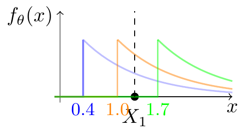
To gain some intuition, imagine that we observe \(X_1 = 1.3\), and consider the PDF Equation 30.4 for \(\theta = 0.4\), \(\theta = 1.0\), and \(\theta = 1.7\).
Visually, we see that the likelihood of \(\theta = 1.0\) is greater than that of \(\theta = 0.4\). This is because the PDF is a decaying exponential, and the exponential has less “space” to decay when \(\theta\) is larger. On the other hand, if \(\theta\) is too large, the likelihood is actually zero, as we see when \(\theta = 1.7\). The sweet spot that maximizes the likelihood is to set \(\theta = X_1\), where the likelihood is nonzero and the exponential has not started to decay.
Now, returning to the setup of the original problem where we have a random sample \(X_1, \dots, X_n\) from this distribution. We want to make \(\theta\) as large as possible but no larger. If we choose a value of \(\theta\) that is greater than some \(X_i\), then the likelihood will be zero. In other words, we want to make \(\theta\) as large as possible, but we also want to ensure that \(\theta \leq \min(X_1, \dots, X_n)\). Therefore, the MLE is \[ \hat\theta = \min(X_1, \dots, X_n). \]
Notice that log-likelihoods and calculus are not helpful in this example. The key to the solution was analyzing where the likelihood is zero, and \(\log(0)\) is not defined. Furthermore, the likelihood is not differentiable at the point that matters most, when \(\theta = \min(X_1, \dots, X_n)\).
However, there is a way to solve for the MLE using mathematical notation. We can write the PDF Equation 30.4 using indicator functions \[ f_\theta(x) = e^{-(x - \theta)} {\bf 1}{\{ x \geq \theta \}} \] so that the likelihood for the entire sample is \[ \begin{align} L_{x_1, \dots, x_n}(\theta) &= \prod_{i=1}^n e^{-(x_i - \theta)} {\bf 1}_{\{ x_i \geq \theta \}} \\ &= e^{- \sum_{i=1}^n x_i + n\theta} \prod_{i=1}^n {\bf 1}_{\{ x_i \geq \theta \}} \\ &= e^{- \sum_{i=1}^n x_i + n\theta} {\bf 1}_{\{ \min(x_1, \dots, x_n) \geq \theta \}}. \end{align} \]
From the first term, it is clear that likelihood can be maximized by making \(\theta\) as large as possible. However, the second term indicates that \(\theta\) cannot be any greater than \(\min(x_1, \dots, x_n)\), or else the likelihood will be zero.
30.3 Exercises
Exercise 30.1 (The likelihood principle) Your friend claims to be an excellent free throw shooter. You would like to estimate the probability \(p\) that they make a free throw. Assume that free throws are independent.
- Suppose they take 16 shots and successfully make 10. Write down the likelihood function \(L_{X=10}(p)\).
- Suppose they take as many shots as necessary until they successfully make 10 free throws. Suppose that it takes \(Y=16\) free throws. Write down the likelihood function \(L_{Y=16}(p)\).
The two likelihood functions above are different, but they are related. How are they related? Why does this imply that the MLE of \(p\) is the same in both cases? Calculate the MLE of \(p\).
Even though the two likelihood functions are different, they both lead to the same inference about \(p\). This is an example of the likelihood principle.
Exercise 30.2 (Rayleigh distribution) Let \(X_1, \dots, X_n\) be a random sample from a Rayleigh distribution with unknown parameter \(\sigma^2\): \[ f_{\sigma^2}(x) = \begin{cases} \frac{x}{\sigma^2} e^{-\frac{x^2}{2\sigma^2}} & x \geq 0 \\ 0 & \text{otherwise} \end{cases}. \] Find the MLE of \(\sigma^2\).
Exercise 30.3 (Power distribution) Let \(X_1, \dots, X_n\) be i.i.d. with PDF \[ f(x) = \begin{cases} (\theta + 1)x^\theta & 0 \leq x \leq 1 \\ 0 & \text{otherwise} \end{cases}, \] where \(\theta\) is unknown. Find the MLE of \(\theta\).
Exercise 30.4 (Uniform distribution) Let \(X_1, \dots, X_n\) be a random sample from a \(\text{Uniform}(0,\theta)\) distribution, where the upper bound \(\theta\) is unknown. Find the MLE of \(\theta\).
Exercise 30.5 (Rate parameter of the double exponential distribution) The double exponential distribution (also known as the Laplace distribution) has PDF \[ f(x) = \frac{1}{2\sigma} \exp\left( -\frac{\lvert x \rvert}{\sigma} \right); \qquad -\infty < x < \infty, \] where the scale parameter \(\sigma\) is unknown. Find the MLE of \(\sigma\).
Exercise 30.6 (Location of the double exponential distribution) Consider a double exponential distribution (Exercise 30.5) with location parameter \(\mu\) (and scale parameter \(1\), for simplicity): \[ f(x) = \frac{1}{2} e^{-\lvert x - \mu \rvert}; \qquad -\infty< x < \infty. \] For an i.i.d. sample of size \(n = 2m + 1\) (i.e., \(n\) is odd), show that the MLE of \(\mu\) is the median of the sample.
Remark. The function \(\lvert x \rvert\) is not differentiable. Once you find an appropriate quantity to minimize, it may help to draw pictures for small values of \(n\) (e.g., \(n=3\)) to understand the behavior of the said quantity.