18 Random Variables

\[ \def\mean{\textcolor{red}{1.2}} \]

The random variables that we have encountered so far, like

your net earnings if you bet $1 on the number 23
the number of friends who draw their own name in Secret Santa

have all been discrete. That is, these random variables can only take on values in a countable set.

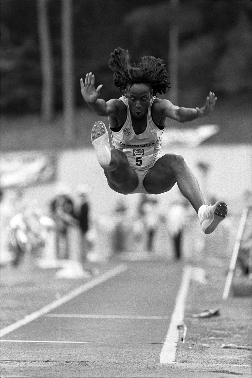
Now, consider a random variable $X$ that represents the distance of one of Jackie Joyner-Kersee’s long jumps (Figure 18.1). Even a professional’s jumps will vary from attempt to attempt; when Joyner-Kersee won gold at the 1988 Seoul Olympics, her three successful long jump attempts were 7.00, 7.16, and 7.40 meters. (The last jump earned her the gold medal and stands as an Olympic record to this day.)

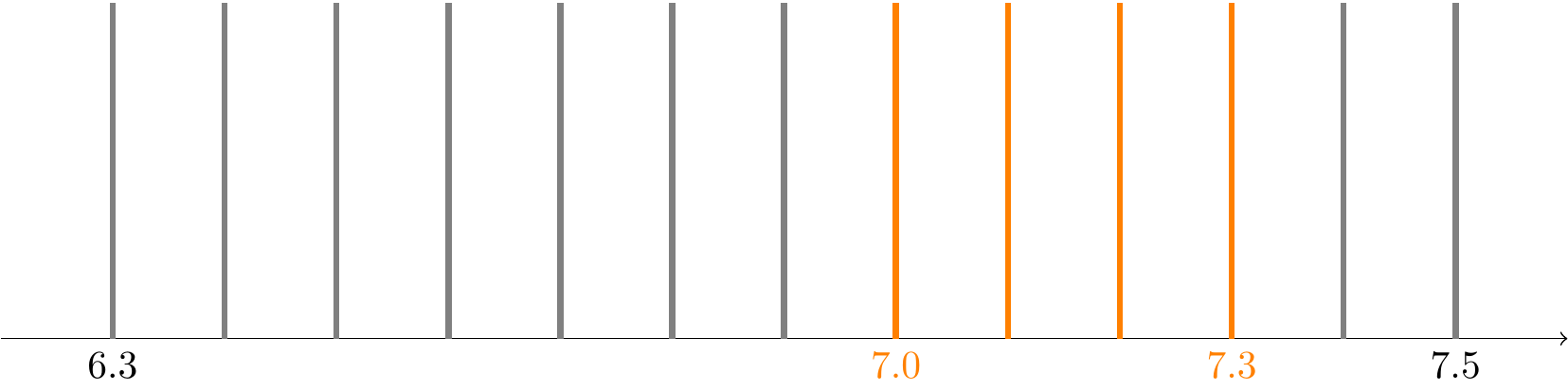
Suppose that we model $X$ as “equally likely” to be any distance between $6.3$ and $7.5$ meters. If we model $X$ at a granularity of $0.1$ meters, then $X$ can be represented as a discrete random variable, whose PDF is shown in Figure 18.2.

Figure 18.1: U.S. track and field Olympian Jackie Joyner-Kersee (source)

Figure 18.2: PMF of $X$, modeled at a granularity of $0.1$ meters. Probabilities corresponding to the event $\{ 7.0 \leq X \leq 7.3 \}$ are highlighted in orange.

The probability $P(7.0 \leq X \leq 7.3)$ is calculated by summing the probabilities highlighted in orange. Since there are 13 possible values, all equally likely, this probability is $\frac{4}{13}$, based on the model in Figure 18.2.

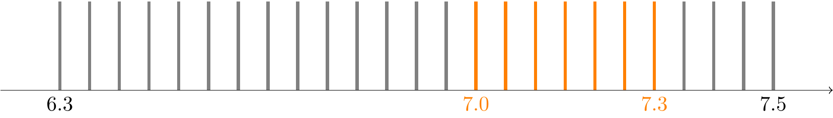
We can improve the precision of our model by increasing the granularity to $0.05$ meters, as shown in Figure 18.3. Now the probability $P(7.0 \leq X \leq 7.3)$ is $\frac{7}{25}$

Figure 18.3: PMF of $X$, modeled at a granularity of $0.05$ meters. Probabilities corresponding to the event $\{ 7.0 \leq X \leq 7.3 \}$ are highlighted in orange.

But there is no reason to stop here. We can always obtain a more precise model by increasing the granularity. As we do so, the probability of each individual value gets smaller and smaller. Nevertheless, the probability of a range of values remains approximately the same.

Figure 18.4: PMF of $X$, modeled at a granularity of $0.02$ meters. Probabilities corresponding to the event $\{ 7.0 \leq X \leq 7.3 \}$ are highlighted in orange.

As we make the model infinitely precise, the probability of each individual value approaches $0$, while the probability of the range $[7.0, 7.3]$ approaches $.25$. This makes sense because this range represents \[ \frac{7.3 - 7.0}{7.5 - 6.3} = .25 \] of the total range of possible values, and all possible values are equally likely.

Clearly, random variables like $X$ cannot be represented by a PMF, since $P(X = c) = 0$ for every value of $c$, yet $P(7.0 \leq X \leq 7.3)$ is not zero. This is like the dartboard example from Chapter 3! The probability that the dart lands on any particular spot is zero, but the probability that it lands somewhere on the dartboard is certainly not zero!

Random variables like $X$, where all real numbers in a range are possible, are called continuous. We will see that the correct way to describe continuous random variables is by a probability density function (or PDF, for short), shown in Figure 18.5.

Figure 18.5: PDF of $X$. The area shaded in orange corresponds to $P(7.0 \leq X \leq 7.3)$.

The PDF $f(x)$ does not represent the probability of the value $x$; after all, for a continuous random variable, this probability is always zero. Instead, probabilities correspond to areas under the PDF. For example, $P(7.0 \leq X \leq 7.3)$ is equal to the area of the orange shaded region in Figure 18.5.

In order to define the PDF formally, we first revisit the cumulative distribution function (CDF), which is well-defined for both discrete and continuous random variables.

18.1 Cumulative Distribution Function

Recall from Chapter 8 that discrete random variables can be described by either their PMF or CDF. Although continuous random variables do not have a PMF, they still have a CDF. Recall from Section 8.3 that the cumulative distribution function of a random variable represents the “probability up to $x$” and is defined as \[ F(x) \overset{\text{def}}{=}P(X \leq x). \]

Example 18.1 (CDF of $X$) Let’s determine the CDF of $X$, how far Joyner-Kersee jumps (in meters) under the “equally likely” model above.

First, consider the case where $x$ is between $6.3$ and $7.5$. The probability that the distance jumped is in the interval $(6.3, x)$ must be proportional to the length of the interval. By the same logic as above, \[ F(x) \overset{\text{def}}{=}P(X \leq x) = \frac{x - 6.3}{7.5 - 6.3}; \qquad 6.3 \leq x \leq 7.5. \]

But what if $x$ is not between $6.3$ and $7.5$ meters?

If $x < 6.3$, then $F(x) = 0$ because the model assumes that she cannot jump less than $6.3$ meters.
If $x > 7.5$, then $F(x) = 1$, since the model assumes that she cannot jump more than $7.5$ meters, so she is guaranteed to jump a distance less than or equal to 7.5.

Putting all these cases together, the CDF can be written as \[F(x) = \begin{cases} 0 & x < 6.3 \\ \frac{x - 6.3}{1.2} & 6.3 \leq x \leq 7.5 \\ 1 & x > 7.5 \end{cases}, \tag{18.1}\] and it looks like this.

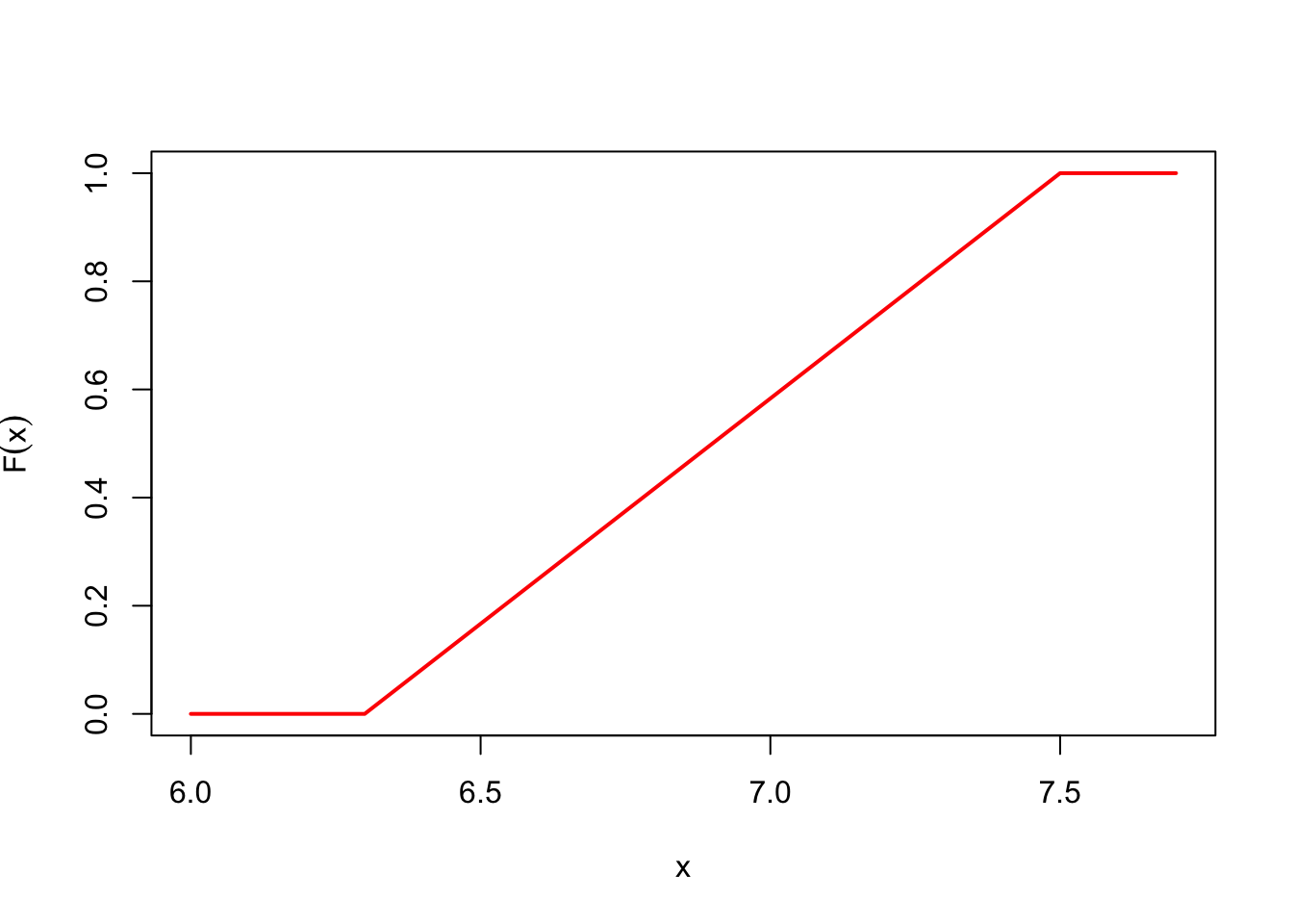
Once we have the CDF, it is straightforward to calculate probabilities by plugging in different values for $x$.

Example 18.2 (Calculating Probabilities Using the CDF) What is the probability that Joyner-Kersee jumps a distance between $7.0$ and $7.3$ meters?

\[ \begin{align*} P(7.0 \leq X \leq 7.3) &= P(X \leq 7.3) - \underbrace{P(X < 7.0)}_{P(X \leq 7.0)} \\ &= F(7.3) - F(7.0) \\ &= \frac{7.3 - 6.3}{1.2} - \frac{7.0 - 6.3}{1.2} \\ &= .25. \end{align*} \]

In the first line, we were able to replace $P(X < 7.0)$ by $P(X \leq 7.0) \overset{\text{def}}{=}F(7.0)$ because the two events only differ by the event $\{ X = 7.0 \}$, and $P(X = 7.0) = 0$.

On a related note, if you were wondering whether “between $7.0$ and $7.3$” includes the endpoints, the answer is that it does not matter! For continuous random variables, the probability that $X$ is exactly $7.0$ or $7.3$ is zero.

All properties of the CDF from Section 8.3 carry over to continuous random variables:

non-decreasing with a left limit of 0 and a right limit of 1, and
right-continuous.

In fact, the CDF of a continuous random variable is not only right-continuous; it is continuous. This is why these random variables are called “continuous” in the first place. Any continuous function $F(x)$ that satisfies these properties is the CDF of a continuous random variable.

18.2 Probability Density Function

In the introduction to this chapter, we introduced the PDF as the analog of the PMF for continuous random variables. Like the PMF, the PDF $f(x)$ indicates which values are more “likely” than others, and is often more intuitive than the CDF. In this section, we define the PDF rigorously using the CDF. But we start with an informal definition of the PDF.

18.2.1 Informal Definition

In the hypothetical PDF shown in Figure 18.6, $f(7.2) > f(6.8)$, so the random variable is more likely to be “near” $7.2$ than $6.8$, even though the probability that it is equal to either value is zero.

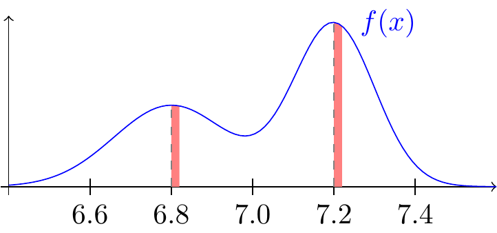
As we will see in Proposition 18.1, probabilities correspond to areas under the PDF. Since there cannot be any area at a single point, $P(X = 6.8)$ and $P(X = 7.2)$ are zero. But $P(6.8 \leq X < 6.81)$ and $P(7.2 \leq X < 7.21)$ are not zero and correspond to the areas of the red shaded regions in Figure 18.6. By comparing these areas, we can determine that

\[ P(6.8 \leq X < 6.81) < P(7.2 \leq X < 7.21). \] For this reason, we say that $X$ is more likely to be “near” $7.2$ than $6.8$.

18.2.2 Formal Definition

Let’s define the PDF more formally. If we want the PDF $f(x)$ to describe the probability that the random variable is “near” $x$, we need the probability that $X$ is in a small interval $[x, x + \varepsilon)$ to be \[ P(x \leq X < x + \varepsilon) \approx f(x) \cdot \varepsilon. \tag{18.2}\] Notice that this probability gets smaller as $\varepsilon$ decreases. This makes sense because as $\varepsilon$ decreases, the probability approaches $P(X = x)$, which is zero for any continuous random variable.

Now, we can rewrite the left-hand side of Equation 18.2 in terms of the CDF so that Equation 18.2 becomes: \[ F(x + \varepsilon) - F(x) \approx f(x) \cdot \varepsilon. \] Next, we divide both sides by $\varepsilon$ and take the limit as $\varepsilon$ approaches 0 (since this is an approximation for $\varepsilon$ small): \[ \begin{aligned} \underbrace{\lim_{\varepsilon\to 0} \frac{F(x + \varepsilon) - F(x)}{\varepsilon}}_{F'(x)} \approx f(x) \end{aligned} \tag{18.3}\]

This is the basis for a rigorous definition of the PDF $f(x)$.

Definition 18.1 (Probability Density Function) The probability density function (or PDF) $f(x)$ of a continuous random variable is the derivative of its CDF:

\[ f(x) = F'(x). \tag{18.4}\]

18.2.3 Examples

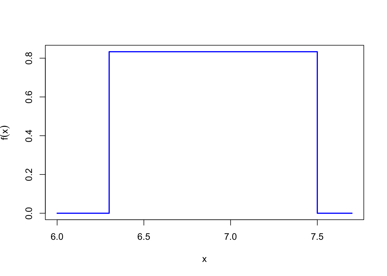
Let’s use Definition 18.1 to determine the PDF of $X$, the distance that Joyner-Kersee jumps under the model above.

Example 18.3 (Determining the PDF of $X$) Starting from the CDF $F$ given by Example 18.1, we calculate the PDF of $X$ using Definition 18.1.

\[ f(x) = F'(x), \]

We calculate this derivative piece by piece. Since \[F(x) = \begin{cases} 0 & x < 6.3 \\ \frac{x - 6.3}{1.2} & 6.3 \leq x \leq 7.5 \\ 1 & x > 7.5 \end{cases},\] we can take the derivative of each case separately to obtain: \[f(x) = F'(x) = \begin{cases} 0 & x < 6.3 \\ \frac{1}{1.2} & 6.3 \leq x \leq 7.5 \\ 0 & x > 7.5 \end{cases},\]

We can simplify the PDF of $X$ to \[ f(x) = \begin{cases} \frac{1}{1.2} & 6.3 \leq x \leq 7.5 \\ 0 & \text{otherwise} \end{cases}, \tag{18.5}\] which was graphed in Figure 18.5.

This PDF makes intuitive sense. It is constant between $6.3$ and $7.5$ meters to reflect the model’s assumption that Joyner-Kersee is equally likely to jump any distance between $6.3$ and $7.5$ meters. It is zero outside of this range because the model assumes that these are the only possible distances. The range where a PDF is non-zero is called the support of the random variable. So the support of $X$ is $[6.3, 7.5]$.

Units of the PDF

What are the units on the vertical axis of Figure 18.5? In other words, what are the units of the PDF? Unlike a PMF, the values of a PDF are not probabilities. Instead, they represent probabilities per unit. In the case of this PDF, the units are “probability per meter”. We can also see this from Equation 18.3; the numerator is a probability, while the denominator is in meters.

We can also calculate probabilities using the PDF directly. The next result follows from Definition 18.1 and the Fundamental Theorem of Calculus.

Proposition 18.1 (Integrate the PDF to Get Probabilities) To calculate the probability that a continuous random variable $X$ falls in some interval $(a, b)$, integrate the PDF $f(x)$ over that interval: \[ P(a < X < b) = \int_a^b f(x)\,dx. \tag{18.6}\]

Proof

Proof. Note that we already know how to calculate the probability using the CDF $F(x)$. \[ \begin{align*} P(a < X < b) &= P(a < X \leq b) & \text{(since $P(X = b) = 0$)} \\ &= P(X \leq b) - P(X \leq a) \\ &= F(b) - F(a). \end{align*}\] Now, since $F$ is the antiderivative of $f$ by Definition 18.1, we can use the Fundamental Theorem of Calculus to conclude that \[ = \int_a^b f(x)\,dx. \]

In other words, areas under the PDF correspond to probabilities. The next example shows how we could have solved Example 18.2 using the PDF.

Example 18.4 (Calculating Probabilities Using the PDF) The probability that Joyner-Kersee jumps a distance between 7.0 and 7.3 meters is equal to the area of the orange shaded region below.

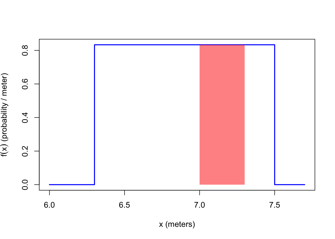
We can calculate the area of the shaded region in two ways:

By geometry, the shaded region is a rectangle with base $(7.3 - 7.0) = .3\ \text{meters}$ and height $\frac{1}{1.2} \frac{\text{probability}}{\text{minute}}$, so the probability is \[ P(7.0 < X < 7.3) = (.3\ \text{meters}) \cdot (\frac{1}{1.2}\ \frac{\text{probability}}{\text{meter}}) = .25.\] Notice how the units cancel to give a probability in the end.
By calculus, the area under the PDF between $7.0$ and $7.2$ is \[ \begin{align*} P(7.0 < X < 7.3) = \int_{7.0}^{7.3} f(x)\,dx &= \int_{7.0}^{7.3} \frac{1}{1.2} \,dx \\ &= \frac{1}{1.2} x \Big|_{7.0}^{7.3} = \frac{1}{1.2} (7.3) - \frac{1}{1.2} (7.0) = .25. \end{align*} \] Note that the second line is just calculus. Probability tells us what integral to set up, but calculus computes the integral. Many students of probability find continuous random variables more challenging, not necessarily because of the probability but because of the calculus.

What is the total area under a PDF, $\int_{-\infty}^\infty f(x)\,dx$? This is just the probability that the random variable is any real number, which is always 1. This means that it is not necessary to include a scale on the $y$-axis; the scale is whatever makes the total area equal to 1.

Together with the requirement that $f(x) \geq 0$ to avoid negative probabilities, this property defines a valid PDF. That is, any function $f(x)$ that satisfies the two properties:

$\int_{-\infty}^\infty f(x)\,dx = 1$
$f(x) \geq 0$

could represent the PDF of a continuous random variable.

We can use Property 1 to determine the scale of the PDF when it is not given, as shown in the next example.

Example 18.5 (Temperature in Iqaluit) In 1999, Canada carved a new territory out of the Northwest Territories to be independently governed by the native Inuit. This new territory, called Nunavut, occupies the northernmost reaches of the Earth.

On the whole, Nunavut is very cold. In the capital, Iqaluit, the high temperature (in Celsius) for a day in May is equally likely to be below freezing as above freezing. More specifically, the daily high temperature $C$ can be modeled as a continuous random variable with PDF

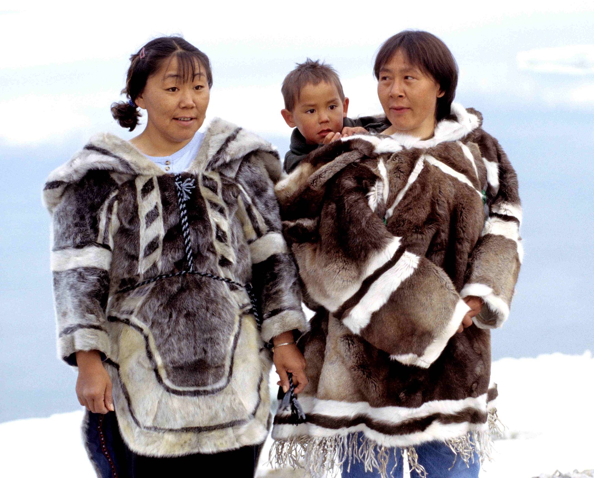
Inuit women and child (source)

\[ f_C(x) = \frac{1}{k} e^{-x^2/18}; -\infty < x < \infty \tag{18.7}\] where $k$ is a constant. Since $k$ is unspecified, we do not know the scale of the PDF. However, we do know that it has the shape shown in Figure 18.7.

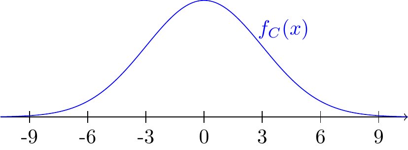
Figure 18.7: PDF of the daily high temperature (in Celsius) in Iqaluit in May

Note that this PDF extends infinitely far in both directions. This reminds us that models like Equation 18.7 are only approximations. As you might remember from chemistry, temperatures cannot be less than absolute zero $(-273.15^\circ C)$, but the probability of that event under this model is so small that it does not affect the practical usefulness of this approximation.

To quote the great statistician George Box, “All models are wrong, but some are useful.” Equation 18.7 can still be a useful model of temperature, even if it is technically wrong.

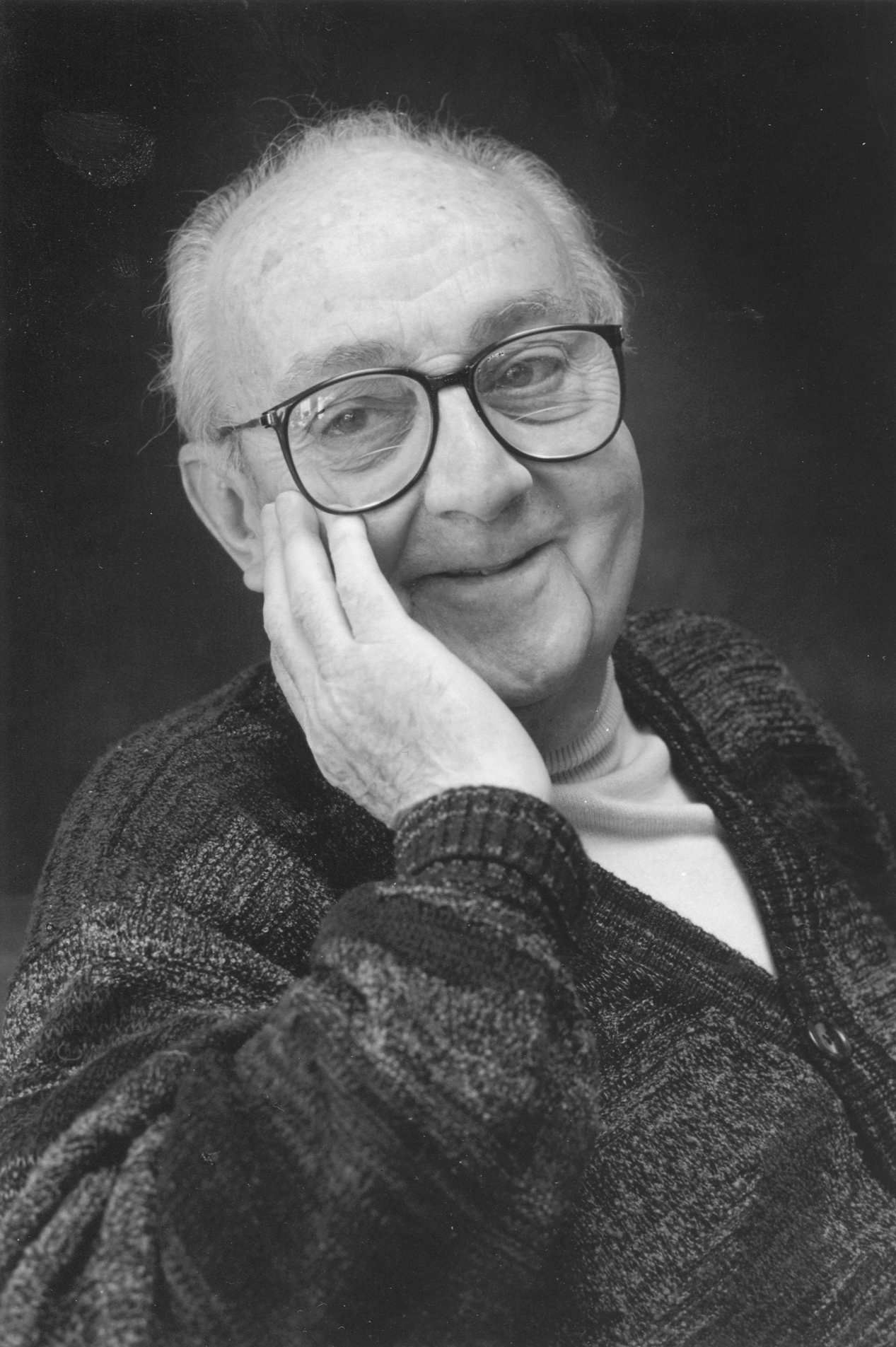
George Box (1919-2013) (source)

To determine the scale $k$, which is called a normalizing constant, we use the property that the total area under any PDF must be 1: \[ \begin{aligned} \int_{-\infty}^\infty \frac{1}{k} e^{-x^2/18}\,dx &= 1 & \Rightarrow & & k &= \int_{-\infty}^\infty e^{-x^2/18}\,dx. \end{aligned} \]

Unfortunately, the expression $e^{-x^2 / 18}$ has no elementary antiderivative, so this integral cannot be evaluated by hand. But we can use R to get a numerical approximation:

So the PDF (Equation 18.7) is approximately \[ f_C(x) \approx \frac{1}{7.519885} e^{-x^2/18}; -\infty < x < \infty. \]

18.3 Case Study: Radioactive Particles

In Example 12.7, we introduced the Geiger counter, a device that measures the level of ionizing radiation. It makes a clicking sound each time an ionization event is detected. The clicks occur at random times, and the times at which they occur is well modeled as a Poisson process. This means that the total number of clicks, counting from time $0$ to time $t$, is a random variable $N_t$, which follows a $\textrm{Poisson}(\mu=\lambda t)$ distribution, where $\lambda$ is the rate of clicks. (The higher the value of $\lambda$, the higher the level of radiation in the air.)

Suppose that we turn on the Geiger counter in a building with $\lambda = \mean$ clicks per minute. Let $T$ be the time of the first click (in minutes), measured from the moment that we turned on the device. In Poisson process lingo, $T$ is called the “first arrival time”.

Example 18.6 (CDF of the First Arrival Time) What is the CDF of $T$?

First, we use the complement rule: \[ F_T(x) = P(T \leq x) = 1 - P(T > x). \] Note that the CDF is zero, unless $x$ is positive.

In words, the event $\{ T > x \}$ means, “The first arrival happened after time $x$.” Another way to say the same thing is “No arrivals happened between time $0$ and time $x$.” Therefore, $\{T > x\}$ is the same event as $\{ N_x = 0 \}$.

This is useful because we know that $N_x$ follows a $\textrm{Poisson}(\mu=\mean x)$ distribution and can calculate this probability. The CDF of $T$ is \[ \begin{aligned} F_T(x) &= 1 - P(T > x) \\ &= 1 - P(N_{x} = 0) \\ &= 1 - e^{-\mean x} \frac{(\mean x)^0}{0!} \\ &= 1 - e^{-\mean x}. \end{aligned} \tag{18.8}\]

Remember that this formula is valid when $x$ is positive. The CDF is zero otherwise. Therefore, $\{ x > 0\}$ is the support of $T$, and we can express the full CDF as \[ F_T(x) = \begin{cases} 1 - e^{-\mean x} & x > 0 \\ 0 & x \leq 0 \end{cases}. \]

Now, we can use Definition 18.1 to derive the PDF from the CDF.

Example 18.7 (PDF of the First Arrival Time) What is the PDF of $T$?

We take the derivative of the CDF (Equation 18.8) to obtain the PDF: \[ \begin{aligned} f_T(x) &= F'_T(x) \\ &= \mean e^{-\mean x}. \end{aligned}\] This formula is valid on the support of $T$, $x > 0$. The PDF is zero elsewhere.

Therefore, we can write the PDF as: \[ f_T(x) = \begin{cases} \mean e^{-\mean x} & x > 0 \\ 0 & \text{otherwise} \end{cases}. \tag{18.9}\]

So what does the PDF Equation 18.9 look like? Let’s graph it.

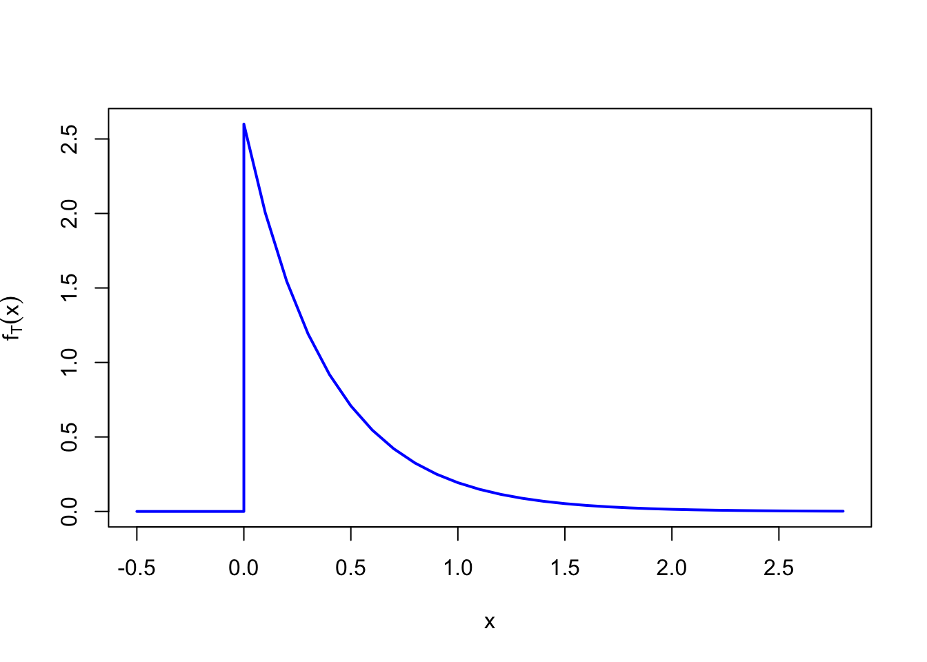
We see that at a rate of $\lambda = \mean$ clicks per minute, the first click is most likely to happen soon after the Geiger counter is turned on, but there is a small (but non-zero) probability that we could be waiting for a long time.

Let’s use the CDF and the PDF to calculate the probability that we need to wait more than 2.3 seconds for the first click.

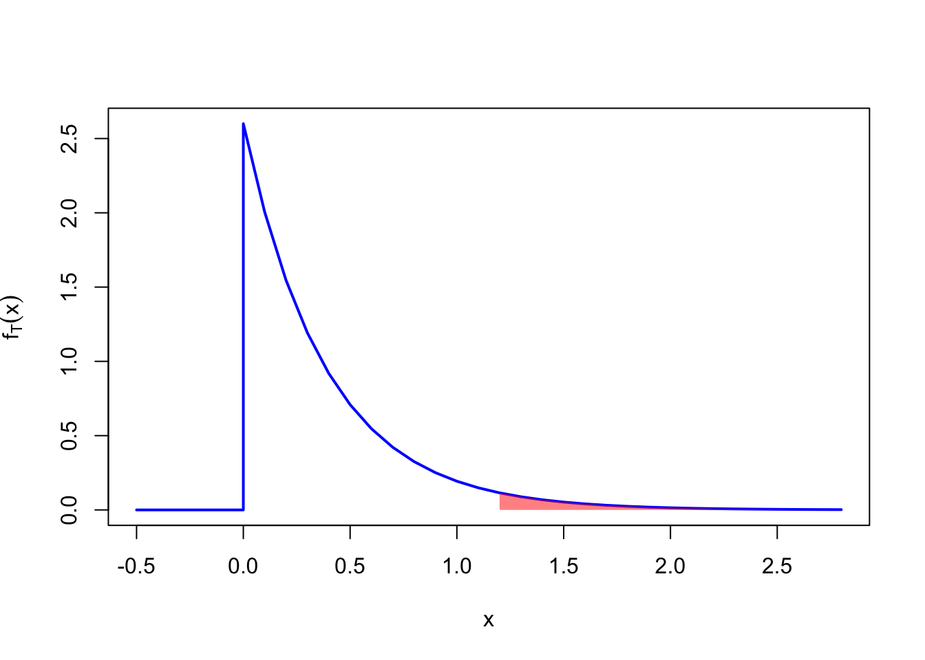
Example 18.8 (Probability of the First Arrival Time) What is the probability that it takes more than $2.3$ seconds for the Geiger counter to register a click?

We can answer this question by plugging $2.3$ into the CDF: \[ P(T > 2.3) = 1 - F_T(2.3) = 1 - (1 - e^{-\mean (2.3)}) \approx .0633 \] or by integrating the PDF from $2.3$ to $\infty$: \[ \begin{aligned} P(T > 2.3) &= \int_{2.3}^\infty \mean e^{-\mean x}\,dx \\ &= -e^{-\mean x} \Big|_{2.3}^\infty = (-e^{-\mean(2.3)}) - (-0) \approx .0633. \end{aligned} \] Once again, it is important to separate the probability (setting up the integral in the first line) from the calculus (computing the integral in the second line). This integral corresponds to calculating the area of the red shaded region below.

Figure 18.9: The probability that the first arrival happens after 2.3 seconds is about 6.3%.

18.4 Calculating the CDF from the PDF

We have seen several examples (Example 18.3, Example 18.7) where we determined the PDF by taking the derivative of the CDF. What if we wanted go in the other direction? We integrate!

Proposition 18.2 (PDF to CDF) To go from the PDF $f(x)$ to the CDF $F(x)$, we integrate: \[ F(x) = \int_{-\infty}^x f(t)\,dt. \]

Proof

By Proposition 18.1, \[ F(x) = P(X \leq x) = P(-\infty < X \leq x) = \int_{-\infty}^x f(t)\,dt. \] Note that because $x$ already appears in the limits of integration, we use $t$ as the variable inside the integral to avoid mixing the two up.

Let’s apply Proposition 18.2 to an example.

Example 18.9 Starting from the PDF $f$ given by Equation 18.5, we determine the CDF of $X$ using Proposition 18.2.

\[ F(x) = \int_{-\infty}^x f(t)\,dt, \] There are three cases:

If $x \leq 6.3$, then $f(t) = 0$ for all $t$ up to $x$, so \[F(x) = 0.\]
If $6.3 < x < 7.5$, then $f(t) = \frac{1}{1.2}$ between $6.3$ and $x$, so \[ F(x) = \int_{6.3}^{x} \frac{1}{1.2}\,dt = \frac{1}{1.2} t \Big|_{6.3}^x = \frac{1}{1.2} (x - 6.3) = \frac{x - 6.3}{1.2}.\]
If $x \geq 7.5$, then we have all of the area between $6.3$ and $7.5$, so \[ F(x) = \int_{6.3}^{7.5} \frac{1}{1.2}\,dt = \frac{1}{1.2} t \Big|_{6.3}^{7.5} = \frac{1}{1.2} (7.5 - 6.3) = 1. \]

Putting the three cases together, we get exactly the CDF $F$ from Equation 18.1.

18.5 Exercises

Exercise 18.1 (Normalizing Constant I) Let \[ f(x) = \begin{cases} \alpha(2x-x^2), & 0 < x < 2 \\ 0, & \text{otherwise} \end{cases}. \]

Find $\alpha$ that makes $f$ a valid PDF.
If $X$ has PDF $f$, compute $P(X < 1.5)$.

Exercise 18.2 (Normalizing Constant II) Let \[ f(x) = \begin{cases} \beta(2x-x^2), & 0 < x < 3 \\ 0, & \text{otherwise} \end{cases}. \]

Is there a $\beta$ that makes $f$ a valid PDF?
If so, compute $P(2 < X < 3)$, if $X$ has PDF $f$.

Exercise 18.3 (When Harry met Sally…) Harry and Sally agree to meet at Katz’s Deli at noon. But punctuality is not Harry’s strong suit; he is equally to arrive any time between 11:50 AM (10 minutes early) and 12:30 PM (30 minutes late). Let $H$ be the random variable representing how late Harry is, in minutes. (A negative value of $H$ would mean that Harry is early.)

What continuous model would be appropriate for $H$? Write down the PDF and CDF of $H$.
Express the event that Harry arrives on time in terms of $H$ and calculate its probability.

Exercise 18.4 (Benford’s Law) Suppose we have quantitative data, such as stock prices or country populations. What does the distribution of first digits look like? That is, what percentage of observations do you expect to start with the digit 1? What about the digit 9?

If you’ve never tried this, look up a list of stock prices or country populations and count how many start with a 1. It may be more than you expect! This phenomenon is called Benford’s Law.

Here is one model that explains Benford’s Law. Suppose the quantitative data can be modeled by a random variable $X$ with PDF \[ f(x) = \begin{cases}\frac{c}{x^2} & x \geq 6 \\ 0 & \text{otherwise} \end{cases}.\]

Determine the value of $c$ that makes this a valid PDF.
Calculate $P(\text{first digit of $X$ is 1})$. (Hint: You will have to calculate the probability of disjoint intervals. These probabilities form a geometric series.)
Calculate $P(\text{first digit of $X$ is 9})$ and compare with your answer to b.