8 Random Variables

In the previous part, we calculated the probability of different events. We described each event as a set of outcomes. It is usually easier to assign a numeric value to each outcome and describe an event in terms of that numeric value. A random variable $X(\omega)$, often abbreviated $X$, is just a function that assigns a numeric value to each possible outcome $\omega$.

8.1 Discrete Random Variables

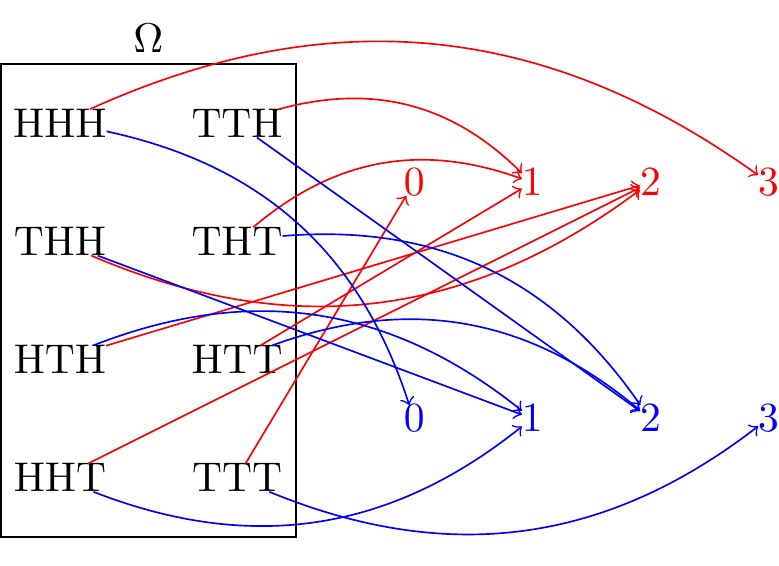
Definition 8.1 (Random variable) Let $\Omega$ be a sample space of an experiment. Then, a random variable $X$ is a function from the sample space $\Omega$ to the real numbers $\mathbb{R}$. In other words, for each outcome $\omega \in \Omega$, $X(\omega)$ is a real number.

Example 8.1 (Heads and tails) Suppose a fair coin is tossed three times. The sample space $\Omega$ is shown below. We can define different random variables on this sample space, depending on what quantity we are interested in:

$\X = \text{the number of heads}$
$\Y = \text{the number of tails}$

Figure 8.1: Two random variables defined on the sample space for three tosses of a fair coin.

That is, the random variable $\X$ is defined as: \[ \X(\omega) = \begin{cases} 0 & \omega \in \{ \text{TTT} \} \\ 1 & \omega \in \{ \text{HTT}, \text{THT}, \text{TTH} \} \\ 2 & \omega \in \{ \text{HHT}, \text{THH}, \text{HTH} \} \\ 3 & \omega \in \{ \text{HHH} \} \\ \end{cases}, \]

while the random variable $\Y$ is defined as: \[ \Y(\omega) = \begin{cases} 0 & \omega \in \{ \text{HHH} \} \\ 1 & \omega \in \{ \text{HHT}, \text{THH}, \text{HTH} \} \\ 2 & \omega \in \{ \text{HTT}, \text{THT}, \text{TTH} \} \\ 3 & \omega \in \{ \text{TTT} \} \\ \end{cases}, \]

It is usually easier to express events of interest in terms of the random variables we define. For example, we can express the event $\{ \text{more heads than tails} \}$ in a number of ways, such as:

$\{ \X \geq 2 \}$ (which is shorthand for $\{ \omega: \X(\omega) \geq 2 \}$)
$\{ \Y \leq 1 \}$
$\{ \X > \Y \}$

So instead of writing $P(\text{more heads than tails})$, we could instead write $P(\X \geq 2)$ or $P(\X > \Y)$.

In general, there are many random variables that we could define on any sample space, and the “right” random variable is the one that helps us solve our problem.

Example 8.2 (Roulette) A classic casino game is roulette. An American roulette wheel consists of 38 pockets, numbered 1-36, 0, and 00, as seen in the picture below.

Picture of a roulette wheel on the left and the betting table on the right

Once all the bets are placed, a ball is spun around the roulette wheel, which eventually settles into one of the 38 pockets.

The sample space for roulette are the 38 pockets that the ball can land in: \[\Omega = \left\{ 0, 00, 1, 2, \dots, 36 \right\}. \]

What is the right random variable for this question? It depends on what bet we make.

Suppose we place a $1 bet on our favorite number, 23. This is called a straight-up bet. If the ball does land in the 23 pocket, we win $35; otherwise we lose the $1 we wagered. We might be interested in the random variable $S$, the profit from this straight-up bet. Note that \[ S(\omega) = \begin{cases} 35 & \omega = 23 \\ -1 & \omega \neq 23 \end{cases} \tag{8.1}\]

The probability that you win with a straight-up bet is only \[ P(S > 0) = \frac{1}{38}. \tag{8.2}\]

Another bet with a higher probability of winning is a bet on reds. If we place a $1 bet on red, and the ball lands any one of the 18 red pockets, we win $1; otherwise, we lose the $1 we wagered. If $R$ is the random variable representing the profit from a $1 bet on reds, then \[ R(\omega) = \begin{cases} 1, & \omega \in \{ 1, 3, 5, 7, 9, 12, 14, 16, 18, 19, 21, 23, 24, 27, 30, 32, 34, 36\} \\ -1, & \omega \in \{ 0, 00, 2, 4, 6, 8, 10, 11, 13, 15, 17, 20, 22, 24, 26, 28, 29, 31, 33, 35 \}\end{cases} \tag{8.3}\] We see that the probability of winning with a bet on reds is \[P(R > 0) = \frac{18}{38}. \tag{8.4}\] There are more chances to win, but the amount we win is less.

All of the random variables we have encountered so far have had a limited set of values. For example, $\X$ and $\Y$ could only assume the values $\{ 0, 1, 2, 3 \}$, while $S$ only took on the values $\{ -1, 35 \}$. These are all examples of discrete random variables. Later, we will see random variables that can assume any value in an interval.

Definition 8.2 (Discrete random variable) A random variable $X$ is said to be discrete if there is a finite list of values $x_1, \dots, x_n$ or a countable list of values $x_1, x_2, \dots$ such that $\displaystyle \sum_i P(X = x_i) = 1$.

8.2 Probability Mass Function

Definition 8.3 (PMF of a discrete random variable) The probability mass function (or PMF) of a discrete random variable $X$ is the function $f_X$ defined as $f_X(x) = P(X = x)$. Note that $f_X$ is a nonnegative function.

Example 8.3 (PMF of the number of heads and the number of tails) In Example 8.1, we defined two random variables:

$\X$, the number of heads in three tosses of a fair coin, and
$\Y$, the number of tails in three tosses of a fair coin.

Because each of the $8$ outcomes in the sample space were equally likely, we can calculate the PMF by simply counting the number of outcomes corresponding to each value and dividing by $8$.

For example, we can calculate the PMF of $\X$ as follows:

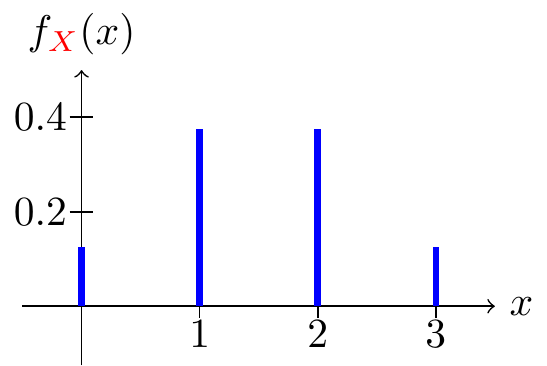
$f_{\X}(0) = P(\X = 0) = \frac{1}{8}$
$f_{\X}(1) = P(\X = 1) = \frac{3}{8}$
$f_{\X}(2) = P(\X = 2) = \frac{3}{8}$
$f_{\X}(3) = P(\X = 3) = \frac{1}{8}$

It is common to lay these probabilities out in a table.

$x$	$0$	$1$	$2$	$3$
$f_{\X}(x)$	$1/8$	$3/8$	$3/8$	$1/8$

The PMF of $\X$ is graphed in Figure 8.2.

Figure 8.2: Visualization of the PMF of $X$

What about the PMF of $\Y$? Verify for yourself that it is the same!

$x$	$0$	$1$	$2$	$3$
$f_{\Y}(x)$	$1/8$	$3/8$	$3/8$	$1/8$

The fact that $\X$ and $\Y$ have the same PMF does not mean that $\X = \Y$. That would mean that the number of heads is always equal to the number of tails. But in fact, this is impossible when a coin is tossed 3 times! There is no outcome $\omega$ for which $\X(\omega) = \Y(\omega)$, so \[ P(\X = \Y) = 0. \]

Example 8.4 (PMF of the profit from a roulette bet) In Example 8.2, we introduced two random variables, $S$ and $R$, which represented one’s profits from $1 bets on 23 and reds, respectively.

The PMF of $S$ is

$x$	$-1$	$35$
$f_{S}(x)$	$37/38$	$1/38$

and the PMF of $R$ is

$x$	$-1$	$1$
$f_{R}(x)$	$20/38$	$18/38$

Notice that the probabilities in any PMF always add up to $1$. This is because events of the form $\{ X = x_i \}$ are a partition of the sample space.

In order for a function $f(x)$ to be a valid PMF, it must satisfy two properties:

$f(x) \geq 0$ for any $x$, and
There need to exist values $x_1, x_2, \dots$ such that $\displaystyle \sum_i f(x_i) = 1$.

In fact, any function $f$ satisfying these two properties is the PMF of some random variable.

8.3 Cumulative Distribution Function

The PMF of a discrete random variable specifies the probability that the random variable is equal to a given value.

There is a related function, the cumulative distribution function (or CDF), which specifies the probability that the random variable is less than or equal to a given value. We can calculate the CDF by summing the PMF over the appropriate values.

Definition 8.4 (CDF of a discrete random variable) The cumulative distribution function (or CDF) of a random variable $X$ with PMF $f$ is the function $F$ defined as \[ F(x) = P(X \leq x) = \sum_{t \leq x} f(t). \]

Example 8.5 (CDF of the number of heads) Using the PMF of $\X$ that we derived in Example 8.3, we can calculate the CDF of $\X$ to be: \[ \begin{aligned} F_{\X}(x) &= \begin{cases} 0 & x < 0 \\ \frac{1}{8} & 0 \leq x < 1 \\ \frac{1}{8} + \frac{3}{8} & 1 \leq x < 2 \\ \frac{1}{8} + \frac{3}{8} + \frac{3}{8} & 2 \leq x < 3 \\ \frac{1}{8} + \frac{3}{8} + \frac{3}{8} + \frac{1}{8} & x \geq 3 \end{cases} \\ &= \begin{cases} 0 & x < 0 \\ \displaystyle \frac{1}{8} & 0 \leq x < 1 \\ \displaystyle \frac{1}{2} & 1 \leq x < 2 \\ \displaystyle \frac{7}{8} & 2 \leq x < 3 \\ 1 & x \geq 3 \end{cases}. \end{aligned} \tag{8.5}\]

This CDF is graphed in Figure 8.3.

Figure 8.3: Visualization of the CDF of $X$

We can use the CDF to quickly evaluate probabilities. For example, to determine the probability we get more heads than tails, $P(\X > 2)$, we can use Equation 8.5 to obtain the answer with almost no calculation: \[ P(\X > 2) = 1 - P(\X \leq 1) = 1 - F_{\X}(1) = 1 - \frac{1}{2} = \frac{1}{2}. \]

Example 8.5 suggests several properties of a CDF:

It is non-decreasing.
As $x$ approaches $-\infty$, $F(x)$ approaches $0$.
As $x$ approaches $\infty$, $F(x)$ approaches $1$.

There is also a simple way to obtain the PMF of a discrete random variable if we already know its CDF.

Example 8.6 (Recovering the PMF from the CDF) Suppose $\X$ is a random variable with the CDF $F(x)$ given in Equation 8.5.

Notice that the CDF jumps at the values $x=0, 1, 2, 3$. For example, the size of the jump at $x=2$ is the difference between \[ F_{\X}(1.9) = P(\X \leq 1.9) = f(0) + f(1) \] and \[ F_{\X}(2.1) = P(\X \leq 2.1) = f(0) + f(1) + f(2), \] which is $f(2)$, the PMF evaluated at $x = 2$.

In other words, the size of each jump at $x$ is precisely the PMF evaluated at $x$, $f(x)$. So we can determine the value of $f(x)$ by calculating the size of each jump at $x$.

At $x = 0$, the CDF jumps from $0$ to $1/8$, so $f(0) = 1/8$.
At $x = 1$, the CDF jumps from $1/8$ to $1/2$, so $f(1) = 1/2 - 1/8 = 3/8$.
At $x = 2$, the CDF jumps from $1/2$ to $7/8$, so $f(2) = 7/8 - 1/2 = 3/8$.
At $x = 3$, the CDF jumps from $7/8$ to $1$, so $f(3) = 1/8$.

This matches the PMF of $\X$ that we derived in Example 8.3.

8.4 Bernoulli and Binomial Random Variables

Suppose we have a coin whose probability of coming up heads is $p$ for some $0 \leq p \leq 1$. Then, we can toss the coin once and define a random variable $X$ as the number of heads in the toss. In other words, if $X = 1$, the coin came up heads, and if $X = 0$, the coin came up tails.

Then, $P(X = 1) = p$ and $P(X = 0) = 1 - p$.

Definition 8.5 (Bernoulli random variable) If $X$ is random variable with the PMF \[ f_X(x) = \begin{cases} p, & x = 1 \\ 1-p, & x = 0 \end{cases} \] for some $0 \leq p \leq 1$, $X$ is said to be a Bernoulli random variable with parameter $p$. We use the notation $X \sim \text{Bernoulli}(p)$.

Suppose we take the same coin and toss it $n$ times, with the outcome of each toss being independent of the other tosses. Let us define a random variable $X$ that counts the number of heads in the $n$ tosses. The possible values of $X$ are $0, 1, \dots, n$.

Now, for some integer $0 \leq k \leq n$, the event $\left\{ X = k \right\}$ means we get $k$ heads (and thus $n-k$ tails) in the $n$ tosses. There are \[ \binom{n}{k} \] configurations of $k$ heads and $n-k$ tails in $n$ tosses – we can think of it as choosing which $k$ of the $n$ tosses will be assigned heads (thereby assigning tails to the $n-k$ tosses not chosen). Each such configuration of $k$ heads and $n-k$ tails has the same probability \[ p^k (1-p)^{n-k} \] of occurring.

Thus, we see that \[ P(X = k) = \binom{n}{k} p^k (1-p)^{n-k}. \]

Definition 8.6 (Binomial distribution) If $X$ is a random variable with PMF \[ f_X(k) = \binom{n}{k} p^k (1-p)^{n-k} \tag{8.6}\] for some $n$ and $0 < p < 1$, $X$ is said to be a binomial random variable with parameters $n$ and $p$. We use the notation $X \sim \text{Binomial}(n,p)$.

Example 8.7 (Coin tosses as binomial) Recall Example 8.3, where we tossed a fair coin three times and $\X$ was the number of heads.

Since each toss is independent, with probability $p = 1/2$ of landing heads, we see that $\X$ matches the template for a $\text{Binomial}(n=3, p=1/2)$ distribution.

Therefore, its PMF can be written as the formula: \[ \begin{aligned} f(k) &= {3 \choose k} (1/2)^k (1 - 1/2)^{3-k}, & 0 \leq k \leq 3. \end{aligned} \tag{8.7}\]

By plugging in $k=0, 1, 2, 3$ into Equation 8.7, we can verify that this formula gives the same probabilities that we calculated in Example 8.3.

$\displaystyle f(0) = {3 \choose 0} (1/2)^0 (1 - 1/2)^{3-0} = \frac{1}{8}$
$\displaystyle f(1) = {3 \choose 1} (1/2)^1 (1 - 1/2)^{3-1} = \frac{3}{8}$
$\displaystyle f(2) = {3 \choose 2} (1/2)^2 (1 - 1/2)^{3-2} = \frac{3}{8}$
$\displaystyle f(3) = {3 \choose 3} (1/2)^3 (1 - 1/2)^{3-3} = \frac{1}{8}$

Even though we motivated the Bernoulli and binomial distributions using coin tosses, these distributions are applicable to far more settings. In order to recognize these applications, we have to map the particular situation onto coin tosses. The following example illustrates how this is done.

Example 8.8 (Phenylketonuria) Phenylketonuria (PKU) is an inherited genetic disorder in humans that results in a decreased ability to process the amino acid phenylalanine. As a result, people with PKU avoid foods that are high in phenylalanine, including egg whites, chicken breast, and the artificial sweetner aspartame. (Many diet sodas have explicit warnings for people with PKU.)

Consider a couple who are both carriers for PKU. That is, they carry the gene for PKU, but they do not have PKU. Mendelian genetics predicts that each of their children has a 25% chance of being born with PKU.

If this couple has 5 children (with no twins), then the number of them who have PKU $X$ is a $\textrm{Binomial}(n= 5, p= .25)$ random variable. To see why, make the analogy with coin tossing:

A coin is tossed $n=5$ times, once for each of the children.
A “heads” means that the child has PKU. This probability is $p=.25$.
Because there are no twins, the children’s genetics are independent. So this situation really is like tossing a coin.

Now that we have established that $X$ is binomial, we can immediately write down its PMF:

\[ f(x) = \binom{4}{x} (.25)^x (1 - .25)^{4-x}; \qquad x=0,1,2,3,4,5. \]

We can plug values into this PMF to obtain the probabilities:

$x$	$0$	$1$	$2$	$3$	$4$	$5$
$f(x)$	$243/1024$	$405/1024$	$270/1024$	$90/1024$	$15/1024$	$1/1024$

We conclude with a probability puzzler that engaged one of the greatest mathematicians of all time.

Example 8.9 (The Newton-Pepys problem) In 1693, Isaac Newton and Samuel Pepys, an English diarist, communicated about the following problem. Pepys wrote Newton a letter asking which of the three has the greatest chance of success:

Six fair dice are tossed independently and at least one six appears.
Twelve fair dice are tossed independently and at least two sixes appear.
Eighteen fair dice are tossed independently and at least three sixes appear.

Pepys thought that option C was the most likely and wanted Newton to verify. We can compute the three probabilities ourselves.

In scenario A, let $X$ denote the number of sixes in six tosses. Then, $X \sim \text{Binomial}(6,1/6)$. The desired probability is \[ P(X \geq 1) = 1 - P(X = 0) = 1 - \binom{6}{0} \left( \frac{1}{6} \right)^0 \left( \frac{5}{6} \right)^6 \approx 0.6651. \] In scenario B, let $Y$ denote the number of sixes in twelve tosses. Then, $Y \sim \text{Binomial}(12,1/6)$. The desired probability is \[\begin{align*} P(Y \geq 2) &= 1 - P(Y = 0) - P(Y = 1) \\ &= 1 - \binom{12}{0} \left( \frac{1}{6} \right)^0 \left( \frac{5}{6} \right)^{12} - \binom{12}{1} \left( \frac{1}{6} \right)^1 \left( \frac{5}{6} \right)^{11} \\ &\approx 0.6187. \end{align*}\] In scenario C, let $Z$ denote the number of sixes in eighteen tosses. Then, $Z \sim \text{Binomial}(18,1/6)$. The desired probability is \[\begin{align*} P(Z \geq 3) &= 1 - P(Z = 0) - P(Z = 1) - P(Z = 2) \\ &= 1 - \binom{18}{0} \left( \frac{1}{6} \right)^0 \left( \frac{5}{6} \right)^{18} - \binom{18}{1} \left( \frac{1}{6} \right)^1 \left( \frac{5}{6} \right)^{17} - \binom{18}{2} \left( \frac{1}{6} \right)^2 \left( \frac{5}{6} \right)^{16} \\ &\approx 0.5973. \end{align*}\]

Newton calculated these odds and correctly concluded that scenario A is the most likely. He also added his intuition that if he imagined scenarios B and C as two and three groups of six tosses, respectively, scenario A requires a six in only one group of six tosses, whereas scenario B would require a six in each of the two groups of six tosses. However, this is incorrect as it is possible to get two sixes in twelve rolls by getting two sixes in the first six tosses and zero sixes in the second six tosses!