In statistics, we typically model data \(Y_1, \dots, Y_n\) as independent random variables. One of the most common models is \[
Y_i \sim \text{Normal}(\mu_i, \sigma^2),
\tag{45.1}\] or equivalently, in random vector notation as \[
\vec Y \sim \textrm{MVN}(\vec \mu, \sigma^2 I).
\]
Note that we do not assume that \(Y_1, \dots, Y_n\) are identically distributed; we allow their means to be different. However, we do assume that they all have the same variance. This assumption, called homoskedasticity (from Greek for “equal scatter”), is essential to simplifying calculations, as we will see.
Here is one situation where we might model data as independent normal, but with different means.
Example 45.1 (Linear regression) Let \(Y_1, \dots, Y_n\) represent the heights of boys ages 5 - 15. We know that children grow taller over time, so if we also know their ages \(x_1, \dots, x_n\), we might model their heights as independent random variables \[
Y_i \sim \text{Normal}(\alpha + \beta x_i, \sigma^2).
\] That is, the mean of each child’s height \(\mu_i \overset{\text{def}}{=}\alpha + \beta x_i\) is a linear function of their age \(x_i\). In other words, it might be reasonable to assume that the heights of the boys are independent normal with the same variance, but with means that increase with age.
If we let \(\vec x \overset{\text{def}}{=}(x_1, \dots, x_n)\), then we can write \(Y_1, \dots, Y_n\) in random vector notation as \[
\vec Y \sim \textrm{MVN}(\vec\mu = \vec 1 \alpha + \vec x \beta, \Sigma = \sigma^2 I).
\]
To estimate \(\alpha\), \(\beta\), and \(\sigma\), we can maximize the (log-)likelihood \[
\ell_{\vec Y}(\alpha, \beta, \sigma^2) = -\frac{n}{2} \log (2\pi \sigma^2) - \frac{1}{2} (\vec Y - (\underbrace{\vec 1 \alpha + \vec x \beta}_{\vec\mu}))^\intercal (\underbrace{\sigma^2 I}_{\Sigma})^{-1} (\vec Y - (\underbrace{\vec 1 \alpha + \vec x \beta}_{\vec\mu})).
\tag{45.2}\]
A bit of algebra shows that the MLEs of \(\alpha\) and \(\beta\) can be obtained by solving \[
(\hat\alpha, \hat\beta) = \underset{\alpha,\beta}{\arg\min}\ \left\| \vec Y - \begin{bmatrix} \vec 1 & \vec x \end{bmatrix} \begin{pmatrix}\alpha \\ \beta \end{pmatrix} \right\|^2,
\] which is a least-squares problem. Once \(\hat\alpha\) and \(\hat\beta\) are found, we set \[
\hat{\vec\mu} = \vec 1 \hat\alpha + \vec x \hat\beta
\] and plug that into Equation 45.2 to obtain the MLE of \(\sigma^2\): \[
\hat\sigma^2 = \underset{\sigma^2}{\arg\max}\ \left( -\frac{n}{2} \log(2\pi\sigma^2) - \frac{1}{2\sigma^2} \left\| \vec{Y} - \hat{\vec{\mu}} \right\|^2 \right).
\] Taking the derivative and setting it to 0 shows \[
\hat\sigma^2 = \frac{1}{n} \Big|\Big|\vec Y - \hat{\vec\mu}\Big|\Big|^2.
\]
In this chapter, we will develop tools for analyzing the sampling distribution of the estimators \(\hat{\vec\mu}\) and \(\hat\sigma^2\).
Projection and Independence
In this section, we will generalize the result from Theorem 44.2. There, we showed that if \(\vec X\) is a vector of i.i.d. \(\text{Normal}(\mu, \sigma^2)\) random variables, then \[ \vec 1 \bar X = P_{\vec{1}} \vec X, \] where \(\displaystyle P_{\vec{1}} \overset{\text{def}}{=}\frac{\vec{1} \vec{1}^\intercal}{n}\), is independent of \[ \vec X - \vec 1 \bar X = (I - P_{\vec{1}})\vec X. \] That result turns out to be true more generally for any (orthogonal) projection matrix \(P\), as well as for independent normal random variables that need not have the same mean (only the same variance).
Definition 45.1 (Orthogonal projection matrix) Let \(P\) be an \(n \times n\) matrix. \(P\) is an orthogonal projection matrix if \(P^2 = P\) and \(P^\intercal = P\).
In particular, \(P\) is the orthogonal projection onto \(C(P) \subseteq \mathbb{R}^n\), where \(C(P)\) denotes the column space of \(P\).
Intuitively, \(P^2 = P\) because the vector is already in the subspace after the first projection, so any subsequent projections do nothing. This property is called idempotence (from Latin for “same power”).
Coming back to \(P_{\vec{1}}\), it has the following properties:
- \(P_{\vec{1}} \vec{1} = \vec{1}\)
- \(P_{\vec{1}} \vec{v} = \vec{0}\) for any \(\vec{v} \in C(\vec{1})^\perp\); i.e., \(\vec{v} \perp \vec{1}\).
Now, we will show that Theorem 44.2 also holds for independent normal random variables that do not necessarily have the same mean, as well as arbitrary projection matrices.
Theorem 45.1 (Independence of projection and residual) As defined as in Equation 45.1, let \[\vec Y = (Y_1, \dots, Y_n) \sim \textrm{MVN}(\vec\mu, \sigma^2 I),\] and let \(P\) be any (orthogonal) projection matrix.
Then, the projection \(P\vec Y\) and the vector of residuals \((I - P)\vec Y\) are independent.
First, note that \[
\begin{pmatrix} P \vec{Y} \\ (I - P)\vec{Y} \end{pmatrix} = \begin{bmatrix} P \\ I - P \end{bmatrix} \vec Y,
\] is multivariate normal by Proposition 44.3. Therefore, if we can show that their cross-covariance is zero, then they must be independent by Theorem 44.1.
\[
\begin{align}
\text{Cov}\!\left[ P\vec Y, (I - P)\vec Y \right] &= P \underbrace{\text{Var}\!\left[ \vec Y \right]}_{\sigma^2 I} (I - P)^\intercal \\
&= \sigma^2 P(I - P) \\
&= \sigma^2 (P - P^2) \\
&= 0_{n \times n}.
\end{align}
\]
Notice that the assumption of homoskedasticity was critical to the proof of Theorem 45.1. If \(\text{Var}\!\left[ \vec Y \right]\) were not proportional to the identity matrix \(I\), then we would not have been able to combine \(P\) and \((I - P)\) to form the zero matrix \(0_{n \times n}\).
Next, we apply Theorem 45.1 to Example 45.1.
Example 45.2 (Independence in linear regression) In Example 45.1, we noted that the MLEs of \(\alpha\) and \(\beta\) could be obtained by solving a least-squares problem: \[
(\hat\alpha, \hat\beta) = \underset{\alpha,\beta}{\arg\min}\ \left\| \vec Y - \begin{bmatrix} \vec 1 & \vec x \end{bmatrix} \begin{pmatrix}\alpha \\ \beta \end{pmatrix} \right\|^2 = \underset{\alpha,\beta}{\arg\min}\ \left\| \vec{Y} - \hat{\vec{\mu}} \right\|^2.
\] The solution is obtained by projecting \(\vec Y\) onto \(\text{span}(\{ \vec 1, \vec x \})\). That is, \[
\hat{\vec \mu} = \underbrace{\begin{bmatrix} \vec 1 & \vec x \end{bmatrix}}_X \begin{pmatrix}\hat\alpha \\ \hat\beta \end{pmatrix} = P_X \vec Y,
\] where \(P_X \overset{\text{def}}{=}X (X^\intercal X)^{-1} X^\intercal\) is the projection matrix onto \(C(X)\). Notice that \(P_X \vec Y\) is a vector representing the “normal” height for each child based on their age.
We also saw that the MLE of \(\sigma^2\) was \[
\hat\sigma^2 = \frac{1}{n} \left\| \vec Y - \hat{\vec\mu} \right\|^2,
\] which can be written as \[
\frac{1}{n} \left\| (I - P_X)\vec Y \right\|^2.
\] \((I - P_X)\vec Y\) is a vector representing how much each child differs from the norm for their age, and \(\hat\sigma^2\) is the average of these squared differences.
By Theorem 45.1, we know that \(P_X\vec Y\) and \((I - P_X)\vec Y\) are independent. Since \(\hat{\vec\mu} = P_X\vec Y\), while \(\hat\sigma^2\) is a function only of \((I - P_X)\vec Y\), they must be independent.
Finally, we make a simple but important observation. If \(P\) is a projection matrix, \((I - P)\) is also. It is also symmetric, and \[
(I - P)^2 = I - 2P + P^2 = I - 2P + P = I - P.
\] In particular, \(P\) is matrix of orthogonal projection onto \(C(P)\), and \(I - P\) is the matrix of orthogonal projection onto \(C(P)^\intercal\).
Length and the Chi-Square Distribution
In this section, we will focus on the case where the data \(Z_1, \dots, Z_n\) are i.i.d. standard normal. That is, \[
\vec Z \overset{\text{def}}{=}(Z_1, \dots, Z_n) \sim \textrm{MVN}(\vec 0, I).
\tag{45.3}\] We will discuss how the results here extend to the more general case (Equation 45.1) at the end.
First, we determine the distribution of the squared length of such a random vector: \[
||\vec Z||^2 = Z_1^2 + Z_2^2 + \dots + Z_n^2.
\] In Section 38.3, we took this to be the definition of a chi-square random variable with \(n\) degrees of freedom, or \(\chi^2_n\), which is identical to the \(\textrm{Gamma}(\alpha= \frac{n}{2}, \lambda= \frac{1}{2})\) distribution.
Now, suppose we multiply \(\vec Z\) by a diagonal matrix \(D\) of the following form: \[
D = \begin{bmatrix} I_{k \times k} \\ & 0_{(n-k) \times (n-k)} \end{bmatrix}.
\tag{45.4}\] Then, \(D\) zeroes out the elements of \(\vec Z\) after the first \(k\) so \[
|| D \vec Z ||^2 = Z_1^2 + \dots + Z_k^2 \sim \chi_k^2.
\tag{45.5}\] This seemingly trivial observation is the basis for a more profound result. It turns out that if \(P\) is any projection matrix onto a subspace of dimension \(k\), then \[
||P\vec Z||^2 \sim \chi^2_k.
\] The argument proceeds as follows:
- The distribution of \(\vec Z\) does not change under rotation; it is still Equation 45.3 in this new coordinate system.
- We can rotate the axes so that the first \(k\) axes span the column space of \(P\). In this new coordinate system, \(P\) is a diagonal matrix of the form Equation 45.4.
- Therefore, the distribution is \(\chi_k^2\) by Equation 45.5.
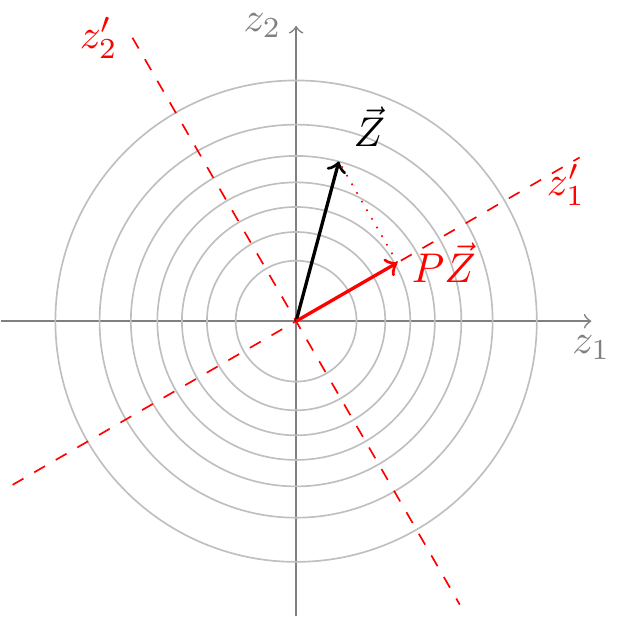
We make this argument precise in Theorem 45.2. However, the essential idea is illustrated in Figure 45.1, which shows the contour lines of the multivariate normal PDF for \(n=2\). (Each line represents a constant value of the PDF.) Because the contour lines are circular, the PDF of \(\vec Z\) does not change if we rotate the axes, so we can choose any axes that are convenient—in particular, we can choose the axes so that the first \(k\) line up with the subspace onto which \(P\) projects. In Figure 45.1, \(P\) projects onto a \(k=1\)-dimensional subspace, and we have chosen \(z'_1\) to line up with this subspace.
In this new coordinate system, \(P\) keeps only the first \(k\) components, zeroing out the remaining \(n-k\) components. That is, in this coordinate system, \(P\) is a diagonal matrix of the form Equation 45.4. Therefore, by the same logic as Equation 45.5, the distribution of \(|| P\vec Z ||^2\) must be \(\chi^2_k\).
The next two results make the above argument precise.
Lemma 45.1 (Rotating a multivariate normal) Let \(Q\) be any orthogonal matrix. That is, the columns of \(Q\) are an orthonormal basis of \(\mathbb{R}^n\) so that \(Q^\intercal Q = I\). Then, \(\vec Z' \overset{\text{def}}{=}Q\vec Z\) has the same distribution as \(\vec Z\). That is, \(\vec Z'\) is also a vector of i.i.d. standard normals.
The distribution of \(\vec Z' \overset{\text{def}}{=}Q\vec Z\) is also multivariate normal by Proposition 44.3. By Proposition 43.1, its mean vector is \[ \text{E}\!\left[ \vec Z' \right] = \text{E}\!\left[ Q\vec Z \right] = Q\text{E}\!\left[ \vec Z \right] = Q \vec 0 = \vec 0 \] and its covariance matrix is \[ \text{Var}\!\left[ \vec Z' \right] = \text{Var}\!\left[ Q\vec Z \right] = Q\underbrace{\text{Var}\!\left[ \vec Z \right]}_{\sigma^2 I} Q^\intercal = \sigma^2 \underbrace{QQ^\intercal}_I = \sigma^2 I, \] which together completely characterize a multivariate normal distribution. So \(\vec Z'\) has the same distribution as \(\vec Z\).
Here is the geometric intuition for this result. The PDF of \(\vec Z\) is \[
f_{\vec Z}(\vec z) = \frac{1}{(2\pi\sigma^2)^{n/2}} e^{-\frac{1}{2\sigma^2} \sum_{i=1}^n z_i^2},
\] which only depends on the distance from the origin, so it is spherically symmetric. On the other hand, the orthogonal matrix \(Q\) is simply a rotation around the origin. So multiplying by \(Q\) may change the value of \(\vec Z\), but does not change its distribution.
Now we are ready to establish the main theorem, which is a special case of a more general result proved by the Scottish-American statistician Bill Cochran. Despite the theoretical nature of this result, Cochran was in fact the consummate applied statistician—for example, serving on the scientific advisory committee for the U.S. Surgeon General’s 1964 report that cigarette smoking causes lung cancer. Cochran served as the chair of the Johns Hopkins Department of Biostatistics, before moving to Harvard to found its the Department of Statistics.
William Cochran (1909-1980)
Theorem 45.2 (Cochran (1934)) Let \(P\) be a rank-\(k\) projection matrix; that is, it projects vectors onto a subspace of dimension \(k\). Then, \[
|| P \vec Z ||^2 \sim \chi_k^2.
\]
Since \(P\) projects onto a subspace of dimension \(k\), we can let \[\{ \vec q_1, \dots, \vec q_k \}\] be an orthonormal basis of this subspace, which exists by the Gram-Schmidt algorithm. Note that all of these vectors are eigenvectors of \(P\) with eigenvalue \(1\) because they are already in the subspace, so \[ P\vec q_j = \vec q_j; \qquad j=1, \dots, k. \]
We can extend this to an orthonormal basis of \(\mathbb{R}^n\). Applying Gram-Schmidt to \(\left\{ \vec{q_1}, \dots, \vec{q_k}, \vec{e_1}, \dots, \vec{e_n} \right\}\) yields \[
\left\{ \vec{q_1}, \dots, \vec{q_k}, \vec{q_{k+1}}, \dots, \vec{q_n} \right\}.
\] Note that \(\left\{ \vec{q_{k+1}}, \dots, \vec{q_n} \right\}\) is an orthonormal basis of \(C(P)^\perp\). Hence,
\[ P\vec q_j = \vec 0; \qquad j=k+1, \dots, n. \]
Therefore, \(PQ = QD\), where \(Q\) is an orthogonal matrix consisting of the eigenvectors \[
Q \overset{\text{def}}{=}\begin{bmatrix} \vert & & \vert & \vert & & \vert \\ \vec q_1 & \dots & \vec q_k & \vec q_{k+1} & \dots & \vec q_n \\ \vert & & \vert & \vert & & \vert \end{bmatrix},
\] and \(D\) is a diagonal matrix consisting of the eigenvalues \[
D = \begin{bmatrix} I_{k \times k} \\ & 0_{(n-k) \times (n-k)} \end{bmatrix}.
\] Equivalently, we can write \(P = QDQ^\intercal\), since \(Q^{-1} = Q^\intercal\).
Substituting this diagonalization into the above, we see that \[
|| P\vec Z ||^2 = || (QDQ^\intercal)\vec Z ||^2 = \vec Z^\intercal (Q D \underbrace{Q^\intercal) (Q}_{I} D Q^\intercal) \vec Z = || D Q^\intercal \vec Z ||^2.
\] But by Lemma 45.1, we know that \(Q^\intercal \vec Z\) has the same distribution as \(\vec Z\), so \(|| D Q^\intercal \vec Z||^2\) must have the same distribution as \(||D \vec Z ||^2 = Z_1^2 + \dots + Z_k^2\), which is \(\chi^2_k\).
Although it is usually unreasonable to assume that data are i.i.d. standard normal, data can often be reduced to standard normal random variables. The next result illustrates one such situation.
Theorem 45.3 (Distribution of the sample variance for normal data) Let \(X_1, \dots, X_n\) be i.i.d. \(\text{Normal}(\mu, \sigma^2)\), and let \(S^2\) be the sample variance. Then,
\[
\frac{(n-1)S^2}{\sigma^2} \sim \chi^2_{n-1}
\]
First, we observe that the random variable in question can be written as \[\begin{align}
\frac{(n-1) S^2}{\sigma^2} &= \frac{\sum_{i=1}^n (X_i - \bar X)^2}{\sigma^2} \\
&= \sum_{i=1}^n \left(\frac{X_i - \mu}{\sigma} - \frac{\bar X - \mu}{\sigma}\right)^2 \\
&= \sum_{i=1}^n (Z_i - \bar Z)^2,
\end{align}\] where \(Z_1, \dots, Z_n\) are i.i.d. standard normal.
Let \(\vec Z \overset{\text{def}}{=}(Z_1, \dots, Z_n)\). Then, we can write \[
\sum_{i=1}^n (Z_i - \bar Z)^2 = || \vec Z - \vec 1 \bar Z ||^2 = ||(I - P_{\vec{1}}) \vec Z||^2.
\tag{45.6}\]
Since \(P_{\vec{1}}\) projects onto a \(1\)-dimensional subspace, \((I - P_{\vec{1}})\) projects onto an \((n-1)\)-dimensional subspace. By Theorem 45.2, \(\left\| (I - P_{\vec{1}})\vec Z \right\|^2\) follows a \(\chi_{n-1}^2\) distribution.
One consequence of Theorem 45.3 is that we can easily determine the bias and variance of \(S^2\) for normal data.
Example 45.3 (Bias and variance of the sample variance) In Proposition 32.2, we showed that the sample variance \(S^2\) is unbiased for the variance \(\sigma^2\) for i.i.d. random variables from any distribution. We can verify this for i.i.d. normal random variables in particular using Theorem 45.3: \[
\text{E}\!\left[ S^2 \right] = \frac{\sigma^2}{n-1} \underbrace{\text{E}\!\left[ \chi_{n-1}^2 \right]}_{n-1} = \sigma^2,
\] where we have abused notation by letting \(\chi_{n-1}^2\) stand in for a random variable with that distribution. The expectation of the \(\chi_{n-1}^2\) distribution follows from the fact that it is another name for the \(\textrm{Gamma}(\alpha= \frac{n-1}{2}, \lambda= \frac{1}{2})\) distribution, whose expectation we know to be \(\alpha/\lambda\).
Similarly, \[
\text{Var}\!\left[ S^2 \right] = \left(\frac{\sigma^2}{n-1}\right)^2 \underbrace{\text{Var}\!\left[ \chi_{n-1}^2 \right]}_{2(n-1)} = \frac{2\sigma^4}{n-1}
\] because the variance of the gamma distribution is \(\alpha/\lambda^2\). However, this formula is only valid when the data are normal; the formula for the variance of \(S^2\) in general is considerably more complicated.
Notice that \(P\vec Z\) in Theorem 45.2 is multivariate normal, with \[
\begin{align}
\text{E}\!\left[ P\vec Z \right] &= P \underbrace{\text{E}\!\left[ \vec Z \right]}_{\vec 0} = \vec 0 & \text{Var}\!\left[ P\vec Z \right] = P \underbrace{\text{Var}\!\left[ \vec Z \right]}_{I} P^\intercal &= P^2 = P,
\end{align}
\] where we used the property of a projection matrix that \(P P^\intercal = P^2 = P\). This immediately implies the following alternative form of Theorem 45.2 that is more general and often more convenient.
Corollary 45.1 (Alternative form of Cochran’s theorem) Suppose \[ \vec W \sim \textrm{MVN}(\vec 0, P). \] Then, \[
|| \vec W ||^2 \sim \chi^2_k.
\]
To see why Corollary 45.1 is more general than Theorem 45.2, consider the distribution of \[
\hat\sigma^2 = \frac{1}{n} ||(I - P_X) \vec Y||^2
\] from Example 45.2. Although \((I - P_X)\) is a projection matrix, \(\vec Y\) does not have zero mean. Nevertheless, we can use Corollary 45.1 to determine the distribution of \(\hat\sigma^2\).
Example 45.4 (Distribution of \(\hat\sigma^2\) in linear regression) Continuing Example 45.2, recall that \[
\vec Y \sim \textrm{MVN}(\vec\mu = \vec 1 \alpha + \vec x \beta, \Sigma = \sigma^2 I).
\]
Therefore, \[
(I - P_X) \vec Y \sim \textrm{MVN}(\underbrace{(I - P_X)\vec\mu}_{\vec 0}, \sigma^2 (I - P_X)),
\] where we used the fact that \(\vec\mu = \vec 1 \alpha + \vec x \beta\) is in the column span of \(X\), so \((I - P_X)\vec\mu = \vec 0\).
Therefore, \[
\hat\sigma^2 = \frac{1}{n} ||(I - P_X) \vec Y||^2 = \frac{\sigma^2}{n} ||\vec W||^2,
\] where \(\vec W \sim \textrm{MVN}(\vec 0, I - P_X)\). Since \((I - P_X)\) is a projection matrix of rank \(n-2\), we can apply Corollary 45.1 to conclude that \[
\frac{n\hat\sigma^2}{\sigma^2} \sim \chi^2_{n-2}.
\] Since chi-square is a special case of the gamma distribution, and a scaled gamma is still a gamma, this is equivalent to \[
\hat\sigma^2 \sim \textrm{Gamma}(\alpha= \frac{n-2}{2}, \lambda= \frac{n}{2\sigma^2}).
\tag{45.7}\]
Here is one useful application of Equation 45.7. Since we know the distribution, we can evaluate its expectation \[
\text{E}\!\left[ \hat\sigma^2 \right] = \frac{\alpha}{\lambda} = \frac{n-2}{n} \sigma^2
\tag{45.8}\] to see that the MLE is biased for \(\sigma^2\). However, Equation 45.8 also suggests the fix. To make the estimator unbiased, we simply need to adjust the scaling: \[
\hat\sigma^2_{\text{unbiased}} = \frac{n}{n-2} \hat\sigma^2 = \frac{1}{n-2} ||\vec Y - \hat{\vec\mu} ||^2.
\]
This is the estimator of variance that is preferred in linear regression, and we now know its sampling distribution: \[
\frac{(n-2) \hat\sigma_{\text{unbiased}}^2}{\sigma^2} \sim \chi^2_{n-2}
\] or equivalently, \[
\hat\sigma_{\text{unbiased}}^2 \sim \textrm{Gamma}(\alpha= \frac{n-2}{2}, \lambda= \frac{n-2}{2\sigma^2}).
\]
Exercises
Exercise 45.1 (Alternative proof of Theorem 45.3) We will prove Theorem 45.3 another way using moment generating functions. Let \(X_1, \dots, X_n\) be i.i.d \(\text{Normal}(\mu, \sigma^2)\) and let \[
S^2 = \frac{1}{n-1} \sum_{i=1}^n \left( X_i - \bar{X} \right)^2.
\]
- First, consider \(Z_1, \dots, Z_n\) be i.i.d. \(\text{Normal}(0,1)\). Show that \[
\sum_{i=1}^n Z_i^2 = \sum_{i=1}^n \left( Z_i - \bar{Z} \right)^2 + n \bar{Z}^2.
\]
- Next, write down the MGF of both sides of the above result to determine the MGF of \[
\sum_{i=1}^n \left( Z_i - \bar{Z} \right)^2.
\] It may be helpful to recall that \(\bar{Z}\) is independent of \(\sum \left( Z_i - \bar{Z}\right)^2\). Use the MGF to determine its distribution.
- Finally, use location-scale transformations \(X_i = \mu + \sigma Z_i\) to conclude that \[
\frac{(n-1) S^2}{\sigma^2} \sim \chi_{n-1}^2.
\]
Exercise 45.2 (Difference of means) Let \(X_1, \dots, X_m, Y_1, \dots, Y_n\) be i.i.d. \(\text{Normal}(\mu, \sigma^2)\).
- What is the distribution of \(\bar X - \bar Y\)?
- Let \(S_X^2\) be the sample variance of \(X_1, \dots, X_m\), and \(S_Y^2\) be the sample variance of \(Y_1, \dots, Y_n\). To estimate \(\sigma^2\), we could use either \(S_X^2\) or \(S_Y^2\), or better yet, we could use the pooled estimate of variance: \[
S_{\text{pooled}}^2 \overset{\text{def}}{=}\frac{(m-1) S_X^2 + (n-1) S_Y^2}{m+n-2}.
\tag{45.9}\] Show that \(S_{\text{pooled}}^2\) is an unbiased estimator of \(\sigma^2\) and determine the exact distribution of \((m+n-2)\frac{S_{\text{pooled}}^2}{\sigma^2}\).
- Argue that \(S_{\text{pooled}}^2\) is independent of \(\bar X - \bar Y\).
In Exercise 46.5, you will use these observations to derive the two-sample \(t\)-test.
Exercise 45.3 (Analysis of variance) Suppose the data is divided into \(K\) independent groups, with group \(i\) consisting of \(n_i\) i.i.d. observations \[ X_{i1}, X_{i2}, \dots, X_{i n_i} \sim \text{Normal}(\mu, \sigma^2). \]
We have assumed that every group has the same mean and variance, but what if we were not sure? One way to test this assumption is to compare the following:
- the between-group sum of squares \(B = \sum_{i=1}^K n_i (\bar X_i - \bar X)^2\) and
- the within-group sum of squares \(W = \sum_{i=1}^K \sum_{j=1}^{n_i} (X_{ij} - \bar X_i)^2\),
where \(\bar X_i\) is the mean of group \(i\) and \(\bar X\) is the overall mean
If \(B\) is much larger than \(W\), then it is reasonable to conclude that the \(K\) groups do not all have the same mean. This is the idea behind a statistical technique called analysis of variance (or ANOVA, for short). In this exercise, you will derive some of the mathematics that underlie ANOVA.
Let \(\vec X = (X_{11}, \dots, X_{1 n_1}, \dots, X_{K1}, \dots, X_{K n_K})\) be the vector of all observations.
- Express \(B = || P_1 \vec X ||^2\) and \(W = || P_2 \vec X ||^2\) for appropriate projection matrices \(P_1\) and \(P_2\).
- Use the representation in (a) to derive the distributions of \(B\) and \(W\).
- Show that \(B\) and \(W\) are independent.
Cochran, William G. 1934. “The Distribution of Quadratic Forms in a Normal System, with Applications to the Analysis of Covariance.” In Mathematical Proceedings of the Cambridge Philosophical Society, 30:178–91. 2. Cambridge University Press.