10 Transformations

In Chapter 8, we saw how the distribution of a random variable can be described by its PMF. We can also transform random variables to obtain new random variables. For example, if $X$ is a random variable, $Y = g(X)$ is a new random variable. How do we describe the distribution of $Y$?

10.1 Functions of a Random Variable

To build some intuition about transformations, we revisit the roulette profits from Example 8.2.

Example 10.1 (Roulette and Transformations) Let $S$ be the profit from a $1 bet on the number 23. We showed in Example 8.2 that the PMF of $S$ is

$x$	$-1$	$35$
$f_{S}(x)$	$37/38$	$1/38$

What if $Y$ represents the profit from a $10 bet on the same number? We can express $Y$ as a transformation $g(S)$; in particular, \[ Y = g(S) = 10 S. \tag{10.1}\]

The possible outcomes are $-10$ and $350$, so the PMF of $Y$ is

$x$	$-10$	$350$
$f_{Y}(x)$	$37/38$	$1/38$

In fact, $S$ itself can be written as a transformation of a simpler random variable $I$, the indicator that the ball lands in the 23 pocket. That is, $I$ is a $\text{Bernoulli}(p=1/38)$ random variable (Definition 8.5), whose PMF is

$x$	$0$	$1$
$f_{I}(x)$	$37/38$	$1/38$

Convince yourself that \[ S = 36 I - 1 \tag{10.2}\] by plugging in $I = 0$ and $I = 1$.

Notice that we can do algebra on random variables. For example, we can derive a formula for $Y$ as a transformation of $I$: \[ Y = 10S = 10(36 I - 1) = 360 I - 10. \]

In the above example, the transformations were all one-to-one. That is, each value of $I$ corresponded to a unique value of $S$, and each value of $S$ corresponded to a unique value of $Y$. When a transformation $Y = g(X)$ is one-to-one, each value $x_i$ of $X$ corresponds to a value $y_i$ of $Y$, and the PMF of $Y$ is simply \[ \begin{align} f_Y(y_i) &= f_X(x_i) \\ &= f_X(g^{-1}(y_i)). \end{align} \] That is, the probabilities do not change; only the locations of those probabilities change.

However, not all transformations are one-to-one. The next example shows an example of a transformation from finance, where multiple values of a random variable $X$ are transformed to the same value of $Y$. In this case, the probabilities do change; to obtain the probability of each value $y_i$ of $Y$, we have to lump the probabilities of the corresponding values of $X$: \[ f_Y(y_i) = \sum_{x: g(x) = y_i} f_X(x). \tag{10.3}\]

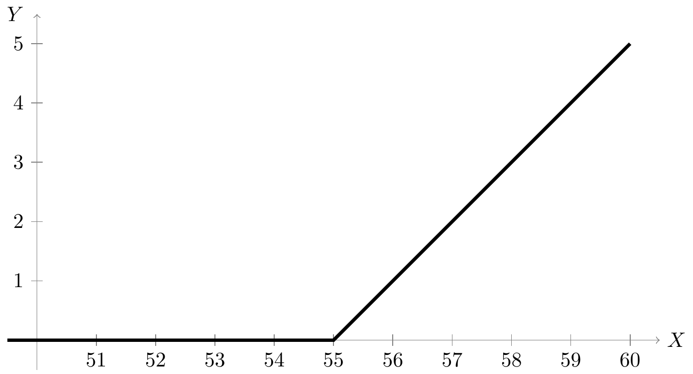
Example 10.2 (Value of a call option) In finance, a call option is a contract that allows the holder to buy a certain share at a pre-determined price (called the “strike price”) at a pre-determined time.

For example, suppose you hold a call option that allows you to buy a stock at a price of $55 in one week. The price of the stock next week is a random variable $X$.

If $X = 53$, then the option is worth nothing because there is no point in exercising the option for $55 when you could just buy the stock for $53.
But if $X = 60$, then the option is worth $5 because $60 - 55 = 5$. (In other words, you could make $5 by exercising the option to buy the stock for $55 and flipping it for $60.)

In other words, the value of this option $Y$ is a transformation of the stock price next week $X$, namely \[ Y = \max(X - 55, 0). \] This function is not one-to-one because any value of $X$ below 55 will map to $Y = 0$.

Figure 10.1: The relationship between $X$ and $Y$.

Suppose the PMF of $X$ is

$x$	$50$	$53$	$57$	$60$
$f_X(x)$	$1/8$	$2/8$	$4/8$	$1/8$

The possible values of $Y$ are $0$, $2$, and $5$. To determine $f_Y(0)$, we need to lump the values of $X$ that map to $Y = 0$:

$f_Y(0) = f_X(50) + f_X(53) = 1/8 + 2/8 = 3/8$.

The other two values of $Y$ each correspond to a single value of $X$, so their probabilities are straightforward:

$f_Y(2) = f_X(57) = 4/8$
$f_Y(5) = f_X(60) = 1/8$.

Therefore, the PMF of the value of the option $Y$ is

$y$	$0$	$2$	$5$
$f_Y(y)$	$3/8$	$4/8$	$1/8$

The next example illustrates how to derive the PMF of a transformed random variable using algebra and by interpreting the random variable.

Example 10.3 (Transformation of a binomial) Suppose $X$ is a $\text{Binomial}(n,p)$ random variable. Define a new random variable $Y$ by $Y = n - X$. In other words, $Y = g(X)$, where $g(x) = n - x$.

We can derive the PMF from $Y$ from the PMF of $X$ using algebra. Note that the two are related by \[ \begin{align} f_Y(y) &\overset{\text{def}}{=}P(Y = y) \\ &= P(n - X = y) \\ &= P(X = n - y) \\ &= f_X(n - y) \end{align} \] for $y = 0, 1, \dots, n$.

Now, substituting $n - y$ into the binomial PMF, we obtain: \[ f_Y(y) = f_X(n-y) = \binom{n}{n-y} p^{n-y} (1-p)^{y} = \binom{n}{y} q^y (1 - q)^{n-y}, \] where $q = 1 - p$. But this is just the PMF of the $\text{Binomial}(n, q)$ distribution.

We could have reached the same conclusion by interpreting the random variables. Recall from Section 8.4 that a binomial random variable $X$ represents the number of heads in $n$ tosses of a coin that has a probability $p$ of coming up heads. In this analogy, $Y = n-X$ would correspond to the number of tails. By relabeling the coin so that tails are “heads” and heads are “tails”, $Y$ represents the number of “heads” (in reality, tails) in $n$ tosses of a coin, with probability $q = 1 - p$ of coming up “heads”, so $Y \sim \text{Binomial}(n, q)$.

The PMF is not the random variable

A common mistake when deriving $f_Y$ is to apply the transformation $g$ to $f_X$ directly. For example, even if $Y = n - X$, \[ f_Y(y) \neq n - f_X(y). \] In fact, this would not even be a valid PMF, as the probabilities would not sum to $1$.

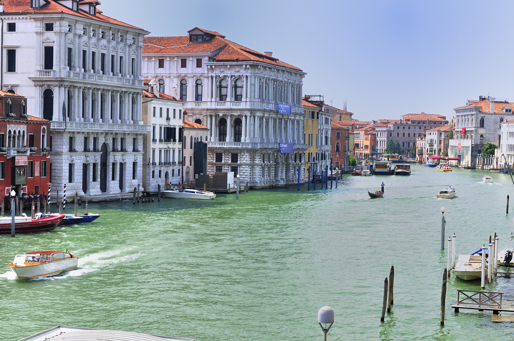
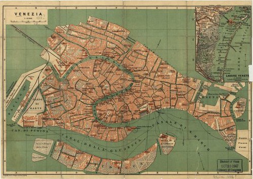
This mistake is symptomatic of a deeper misunderstanding about the distinction between a random variable and its PMF. A random variable is like the city of Venice, and a PMF is like a map of Venice. In the real Venice, you can ride a gondola, drink a spritz, and get lost in the narrow streets. A map of Venice is a representation of the city, and it may help you find your way, but studying a map is not the same as experiencing Venice.

Similarly, a random variable represents a numerical quantity that is random, such as the profit from a roulette bet or the price of a stock next week, while a PMF is a representation of the random variable. If we transform the random variable, the PMF will also change—but not necessarily in the same way. If the city of Venice builds a new bridge, then the map of Venice will also need to be updated, but with pens and ink, not picks and shovels.

In philosophy, the distinction between a thing and its representation is known as the map-territory relation, deriving from Alfred Korzybski’s famous quote, “The map is not the territory.”

10.2 Functions of Multiple Variables

A random variable can also be a transformation of more than one random variable.

Example 10.4 (Sum of independent binomials) Let $X$ and $Y$ be independent $\text{Binomial}(n, p)$ and $\text{Binomial}(m, p)$ random variables, respectively. We will define independence formally in Definition 13.2, but intuitively it means that the value of $X$ gives no information about the value of $Y$.

What is the distribution of $T = X + Y$? Note that this transformation involves multiple random variables.

We can derive the PMF of $T$ using algebra: \[ \begin{align} f_T(t) &\overset{\text{def}}{=}P(T = t) \\ &= P(X + Y = t) & \text{(definition of $T$)} \\ &= P\left( \bigcup_{x=0}^t \{ X = x, Y = t - x \} \right) & \text{(rewrite event)} \\ &= \sum_{x=0}^t P(X = x, Y = t - x) & \text{(disjoint events)} \\ &= \sum_{x=0}^t \underbrace{P(X = x)}_{f_X(x)} \underbrace{P(Y = t - x)}_{f_Y(t - x)} & \text{(independence)} \\ &= \sum_{x=0}^t \binom{n}{x} p^x (1 - p)^{n-x} \binom{m}{t - x} p^{t - x} (1 - p)^{m - (t - x)} & \text{(binomial PMF)} \\ &= \left[\sum_{x=0}^t \binom{n}{x} \binom{m}{t - x}\right] p^t (1 - p)^{n + m - t} & \text{(simplify)} \\ &= \binom{n + m}{t} p^t (1 - p)^{n + m - t}, \end{align} \] where in the last step we used Vandermonde’s identity (Exercise 2.19). This is the PMF of a $\text{Binomial}(n + m, p)$ random variable.

However, it is much easier to reason about the distribution of $T$ by interpreting the random variables. $X$ represents the number of heads in $n$ tosses of a coin, and $Y$ represents the number of heads in $m$ additional tosses (because it is independent of $X$) of the same coin (because the probability $p$ is the same). Therefore, $X + Y$ must represent the number of heads in $n + m$ tosses of the coin, which describes a $\text{Binomial}(n + m, p)$ random variable.

We emphasize once again that the transformations of the random variables are not the same as the operations that we apply to their PMFs. In Example 10.4, we added the random variables $X$ and $Y$, but the operation on their PMFs was \[ f_T(t) = \sum_{x=0}^n f_X(x) f_Y(t - x). \] The operation we are applying to the PMFs is called a convolution, which we will discuss more extensively in Chapter 33.

Example 10.5 (Sum of non-independent binomials) In Example 10.4, it was crucial that $X$ and $Y$ be independent. To see why this is necessary, let $Y = X$, so that both $X$ and $Y$ are $\text{Binomial}(n, p)$ random variables.

Then, \[ T \overset{\text{def}}{=}X + Y = X + X = 2X, \] which is not a binomial random variable. One way to see that it is not binomial is to observe that $2X$ is always an even number. Since there is no reason for a coin to always land heads an even number of times, $T$ does not fit the description of a binomial random variable.

At the risk of beating a dead horse, we reiterate that a transformation like $T = 2X$ is not the same as the operation that we apply to the PMF. That is, \[ f_T(t) \neq 2 f_X(t). \] This would not even be a valid PMF because it would sum to $2$, not $1$.

Finally, we note a useful way to represent the binomial distribution that follows directly from Example 10.4.

Example 10.6 (Sum of independent Bernoullis) Let $X_1, X_2, \dots, X_n$ be $n$ independent $\text{Bernoulli}(p)$ random variables. What is the distribution of $Y = X_1 + X_2 + \cdots + X_n$?

Equivalently, each $X_i$ is a $\text{Binomial}(n=1, p)$ random variable. Now,

$T_2 = X_1 + X_2$ is $\text{Binomial}(n = 2, p)$ by Example 10.4,
$T_3 = \underbrace{X_1 + X_2}_{T_2} + X_3$ is $\text{Binomial}(n = 3, p)$ by the same result,
$T_4 = \underbrace{X_1 + X_2 + X_3}_{T_3} + X_4$ is $\text{Binomial}(n = 4, p)$,

and so on, establishing that \[ Y = X_1 + \dots + X_n \sim \text{Binomial}(n, p). \]

10.3 Exercises

Exercise 10.1 (Value of a put option) A “put option” is like a call option (Example 10.2), except that it allows the holder to sell a certain share at the “strike price” at a pre-determined time.

Consider a put option that allows you to sell the stock in Example 10.2 at a price of $54 next week. Let $X$ be the price of the stock next week.

Argue that the value of the put option is $V = \min(54 - X, 0)$.
Assuming that the stock price $X$ has the same PMF as in Example 10.2, determine the PMF of $V$.

Exercise 10.2 (Transforming a Bernoulli) Let $Y$ be a random variable that only has two possible values, $a$ and $b$. (Assume $a < b$.)

Define a Bernoulli random variable $I$, and a transformation $g$ such that $Y = g(I)$.

Exercise 10.3 (Alternative definition of the geometric distribution) Some books define the geometric distribution differently from this book. They define the geometric distribution as the number of tails (rather than the number of tosses) until a heads is tossed.

Let $Y$ be the number of tails until a heads is tossed. Express $Y$ as a transformation of a suitable geometric random variable $X$. (Recall the definition of a geometric random variable in Definition 8.7.)
Find the PMF of $Y$.

Exercise 10.4 (Surprise) Let $X$ be a random variable with PMF $f$. The surprise of $X$ is defined as \[ S = -\log_2 f(X). \] In other words, we observe a value of $X$, and the smaller the probability of this value, the more “surprised” we are. (We use a base-2 logarithm so that surprise is measured in bits.)

To be concrete, suppose a fair coin is tossed 4 times, and let $X$ be the number of heads.

Is the surprise a one-to-one transformation of $X$?
Calculate the PMF of $S$.