1 Naive Definition of Probability
It’s 1964 in Los Angeles. A blonde-haired woman with a ponytail snatches another woman’s handbag. She flees the scene, but is spotted entering a yellow car driven by a Black man with a beard and a mustache. Later, you spot a woman with blonde hair in a ponytail sharing a yellow car with a bearded and mustachioed Black man. Is this a coincidence? Or, given the extensive set of matching characteristics, is this sufficient evidence to implicate the couple you’ve spotted?
This exact situation was the subject of the famed court case People v. Collins. The prosecution contended that the probability of such a couple existing was so astronomically low (one in 12 million) that the accused must be the actual culprits. The argument compelled the jurors, who reached a guilty verdict. The case was then appealed to the California Supreme Court, where the defense pointed out that the relevant probability was not that of such a couple existing, but that of more than one such couple existing. If multiple such couples existed, the prosecution couldn’t be sure that the accused was the guilty party. For a city the size of Los Angeles, the defense computed this later probability to over 40% (even while using the prosecution’s questionable and unfavorable assumptions). Persuaded by the defense’s argument, the court felt there was insufficient evidence to implicate the accused and overturned the guilty verdict.
Probability theory, the subject of this book, provides a mathematical framework for reasoning about and making decisions under uncertainty. Probabilities allow us to quantify the randomness in real-world systems. We encounter probability statements in everyday life, such as:
- A weather forecaster informs you that there’s a 30% chance of rain tomorrow.
- A betting agency offers 3 to 2 odds that your favorite sports team will win today’s match.
- A friend tells you they’re 90% sure they’ll be free for dinner on Friday.
Also, the ability to quantitatively reason about uncertainty is crucial in many high-impact fields. We provide just a few examples below:
- Finance: Financial analysts are tasked with forecasting the value of financial instruments (e.g., stocks, options, futures) whose day-to-day price movements largely appear random.
- Epidemiology: When studying the spread of infectious diseases, epidemiologists incorporate the stochastic nature of disease transmission into their models.
- Actuarial Science: To appropriately price insurance policies, actuaries must reason about the unknown number of legitimate claims that will be filed in the coming years.
- Law: As we’ve seen in law, prosecutors must establish guilt of the defendant beyond reasonable doubt, i.e., leaving (approximately) no room for uncertainty.
The impacts of these judgments can range from millions of dollars to millions of lives.
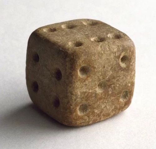
Yet probability theory has origins in a more frivolous, but timeless, endeavor: games. Although games of chance are as old as civilization itself (Figure 1.1 shows a 4000-year old die that looks surprisingly modern), it was not until the 16th century that the games were analyzed systematically.
1.1 A Need for a Mathematical Framework
A brief biography of Gerolamo Cardano
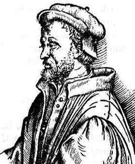
Gerolamo Cardano (1501-1576) was an Italian mathematician. He is best known for his 1545 book Ars Magna, in which he introduced negative and imaginary numbers.
In the same book, he published formulas for the roots of cubic and quartic polynomials. These formulas generalize the familiar quadratic formula, which tells us that \(x = \frac{-b \pm \sqrt{b^2 - 4ac}}{2a}\) gives the roots of the quadratic polynomial \(ax^2 + bx + c\), to 3rd and 4th degree polynomials.
One of the first people to analyze games of chance (and hence, one of the fathers of probability theory) was Gerolamo Cardano (1501-1576). In 1564, Cardano wrote a book, Liber de ludo aleae (“Book on Games of Chance”), in which he analyzed problems like the following.
Although Cardano’s solution sounds plausible, we will see that it is incorrect. It turns out that \(k=3\) throws gives only a 42.1% chance of at least one six, and it takes \(k=4\) throws to achieve a better than 50% chance.
A brief biography of Gottfried Leibniz
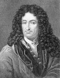
Gottfried Leibniz (1646 -1716) was a German mathematician. He is best known for developing differential and integral calculus, contemporaneously with but independently of Isaac Newton.
Another early pioneer in probability theory was Gottfried Leibniz (1646-1716). Leibniz is best remembered today as the co-inventor of calculus (with Isaac Newton). Leibniz is also attributed with documenting the first modern binary number system, an achievement for which some consider him to be the first computer scientist and information theorist. His far reaching accomplishments have led to him being labeled as the “last universal genius”.
Leibniz, the brilliant 17th century mathematician who co-invented calculus with Isaac Newton, also dabbled in probability theory. In his Opera Omnia (“Complete Works”), he studied the following question.
Leibniz’s solution is also wrong, and his mistake is perhaps easier to spot (we point it out later, but see if you can spot it now!). Interestingly, a similar but harder problem (see Exercise 2.1) was correctly answered by renowned astronomer and scientist Galileo Galilei (1564-1642). Had Leibniz been aware of Galileo’s solution, he likely wouldn’t have made this famed mistake!
A brief biography of Jean le Rond d’Alembert
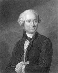
Jean le Rond d’Alembert (1717 -1783) was a French mathematician who is best known for d’Alembert’s principle, a fundamental statement about the classical laws of motion. He also invented the ratio test for the convergence of a series and is known for his work on the fundamental theorem of algebra, which is sometimes called d’Alembert’s theorem in honor of his pioneering attempt to prove it.
Another famed erroneous probability calculation is that of French physicist and mathematician Jean le Rond d’Alembert (1717-1783). D’Alembert studied the following problem in his 1754 article Croix ou Pile (“Heads or Tails”).
D’Alembert’s idea to consider the proportion of outcomes where a heads appears was reasonable and in line with contemporary methods. Unfortunately, as we will see, it wasn’t executed correctly.
Our purpose in recounting these historical blunders is three-fold. First, it emphasizes that probability needs a mathematical foundation. If, over the span of hundreds of years, history’s greatest minds incorrectly computed probabilities when relying on intuition alone, we likely will too. Second, it reminds us how far probability theory has come, and how grateful we should be to enjoy the fruits of its development. By the end of this chapter we’ll fully understand Leibniz’s and d’Alembert’s errors, and by the end of the next we’ll be able to compute the probabilities that eluded Cardano. Lastly, and most importantly, these examples illustrate that probability can be tricky. If Leibniz, who invented a subject as complex as calculus, could botch a basic probability calculation, then we might all struggle with the subject. As you go through this book, don’t be discouraged if concepts seem challenging or counterintuitive at first. With enough practice, anyone can master probability theory!
1.2 A Naive Definition of Probability
A brief biography of Jacob Bernoulli
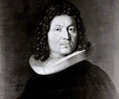
Jacob Bernoulli (1654 - 1705) was a Swiss mathematician. He was an early luminary in a family whose lineage boasts many notable academics. Bernoulli made a number of important contributions to mathematics, including helping found the calculus of variations and discovering the mathematical constant \(e\).
Bernoulli is most famed, however, for his contributions to probability theory. His article Ars Conjectandi, published 8 years after his death, included a derivation of the binomial distribution (discussed in Chapter 8) and, most importantly, the first law of large numbers. Bernoulli, who spent 20 years attempting to prove this law, referred to it as his “golden theorem”. The Bernoulli distribution (also discussed in Chapter 8) is aptly named in his honor.
Jacob Bernoulli’s 1713 posthumous article Ars Conjectandi (“The Art of Conjecturing”) provided the first mathematically rigorous treatment of probability theory. Although limited by today’s standards, Bernoulli’s treatment is still incredibly insightful and powerful. It will allow us to correctly reason about non-trivial problems, including the ones that duped Cardano, Leibniz and d’Alembert.
Bernoulli’s definition considers an experiment that has a finite number of random, but equally likely, outcomes.
An event \(A\) “happens” whenever the experiment’s actual realized outcome belongs to the subset \(A\). Our interest lies in determining the probability of whether particular events will happen or not.
We provide a couple more examples of experiments, sample spaces, and events below. They further illustrate that, although Bernoulli’s formalization is mathematical, these objects are still best understood and most easily discussed in plain English. For the remainder of the book, when we describe something as being random or happening randomly, it means that the different outcomes are equally likely. There are plenty of situations where random outcomes are not equally likely (you’ll see some later in this chapter), and we’ll avoid any confusion by explicitly specifying whenever this is the case.
Within this framework, Bernoulli defines the probability of an event to be the ratio of the number of outcomes in the event to the total number of outcomes in the sample space.
What exactly is the probability \(P(A)\) meant to represent? For now we’ll adopt the frequentist viewpoint. Frequentists believe that probabilities should measure the long run frequencies of random events. A frequentist would find Bernoulli’s formalization suitable if, as we repeat the experiment again and again, the proportion of experiments in which the event \(A\) happens approaches \(P(A)\). We elaborate more on frequentism and contrast it to Bayesianism, which offers a totally different interpretation of probabilities, in Chapter 3.
Equipped with Definition 1.4, we can revisit our earlier examples and compute some probabilities.
1.3 More Examples
Even with just Bernoulli’s naive definition of probability, we can make reasonable quantitative judgements about a number of interesting problems involving chance and uncertainty.
Our first example comes from craps, a game of chance played with dice. We provide a brief introduction to craps for those who are unfamiliar with the game.
A brief introduction to craps
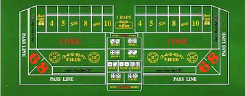
Craps is gambling game played by repeatedly rolling a pair of fair six-sided dice. If the come out roll (the first roll) is a \(2\), \(3\), \(7\), \(11\), or \(12\), the game ends immediately. Otherwise, the come out roll (which must be a \(4\), \(5\), \(6\), \(8\), \(9\), or \(10\)) is set as the point, and the shooter (person rolling the dice) keeps rolling until they either seven out, meaning they roll a \(7\), or they roll the point again.
We consider just a couple of the many bets players can make:
Pass-line bet: A pass line bet pays \(\$1\) for every \(\$1\) wagered. The bettor wins automatically if the come out roll is a \(7\) or \(11\) and loses automatically if it is a \(2\), \(3\), or \(12\). Otherwise, the bettor wins if the shooter rolls the point again before sevening out.
Don’t pass bet: A don’t pass bet also pays \(\$1\) for every \(\$1\) wagered, but it is almost the opposite of a pass-line bet. The bettor wins automatically if the first roll is a \(7\) or \(11\) and loses automatically if it is a \(2\), \(3\). When the come out roll is a \(12\), there is a push (a tie) and the bettor is simply returned their wager with no profit. Otherwise, the bettor wins if the shooter sevens out before rolling the point again.
Example 1.8 (Winning a pass-line bet on the come out roll) If we make a pass-line bet in craps, what’s the probability of winning on the come out roll?
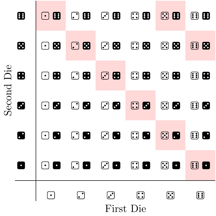
We’ll treat the game of craps as our “experiment” and imagine that one of the dice we’re playing with is black and the other is white. Since we only care about the come out roll, we can denote all the possible outcomes as \((x, y)\) where \(x\) is black die’s value on the come out roll and \(y\) is the white’s. The sample space \(\Omega\), depicted in Figure 1.7, then contains \(36\) equally likely outcomes: all possible pairs \((x, y)\) where \(x = 1,\dots, 6\) and \(y = 1, \dots, 6\).
The event \(A\) of winning a pass-line bet on the come out roll contains exactly the outcomes \((x, y)\) such that \(x + y = 7\) and \(x + y = 11\). Figure 1.7 highlights all the outcomes in \(A\):
\[ A = \{(1, 6), (6, 1), (5, 2), (2, 5), (3, 4), (3, 4), (5, 6), (6, 5)\}. \]
Therefore, the probability of winning on the come out roll is
\[ P(A) = |A|/|\Omega| = 8/36 = 2/9. \]
We can now also correctly solve Leibniz’s problem and identify his mistake.
In both our study of craps (Example 1.8) and Lebniz’s problem (Example 1.9), we were interested in the sum of the two rolled dice. Why then did we parameterize our sample space in terms of the individual die rolls rather than their sum? Why not use the sample space \(\Omega = \{2, \dots, 12\}\)?
Bernoulli’s definition of probability (Definition 1.4) is only reasonable if the outcomes in our sample space are equally likely. When using it, we need to be careful to pick a sample space for which that is the case. Otherwise, as the below example illustrates, it can lead to some nonsensical conclusions.
In the case of rolling two dice, there’s no basis for assuming that the different possible sums of the two rolled dice are equally likely. Conversely, the dice’s symmetric build and the manner in which they are tossed support the assumption that the the outcomes in Figure 1.7 should be.
Failing to recognize that certain outcomes were not equally likely was exactly d’Alembert’s mistake.
Our last example considers a tricky card game that we wager would still fool some great minds today.
Even after working carefully through Example 1.12, it may be difficult to spot the flaw in the gambler’s purposefully misleading reasoning. But worry not! We’ll clearly pinpoint this flaw in Chapter 5 when we cover conditional probabilities. We’ll even be able redo Example 1.12’s analysis without specifying the gambler’s strategy.
1.4 Exercises
Coming soon!