Lesson 9 Bayes’ Theorem
9.1 Motivating Example
The ELISA test is used to screen blood for HIV.
- When the blood contains HIV, it gives a positive result 98% of the time.
- When the blood does not contain HIV, it gives a negative result 94% of the time.
The prevalence of HIV is about 1% in the adult male population. A patient has just tested positive and wants to know the probability that he has HIV. What would you tell him?
The solution to this problem involves an important theorem in probability and statistics called Bayes’ Theorem. This video covers some of the intuition and the history behind Bayes’ Theorem. Don’t worry about the details for now. This video is meant to be more inspiring than informative.
9.2 Theory
The conditional probabilities \(P(A | B)\) and \(P(B | A)\) are not the same. For example, let \(A\) be “currently a Cal Poly student” and \(B\) be “went to high school in California”.
- \(P(B | A)\) is very high, about \(0.85\), since most Cal Poly students are in-state.
- \(P(A | B)\) is very low, as only a very small fraction of people who went to high school in CA are currently in college, much less at Cal Poly.
Bayes’ Theorem is a way to convert probabilities of the form \(P(B | A)\) into probabilities of the form \(P(A | B)\). This switcheroo is surprisingly common in probability and statistics. For example,
- Doctors know the probability that a patient tests positive (\(B\)) given that they have the disease (\(A\)), but a patient is more interested in the probability that he has the disease (\(A\)) given that he tested positive (\(B\)).
- E-mail providers can collect data on the probability that an e-mail contains a certain word (\(B\)) given that it is spam (\(A\)), but a spam filter needs the probability that the e-mail is spam (\(A\)) given that it contains the word (\(B\)).
Don’t be deceived by its simplicity; Bayes’ Theorem is one of the most important and powerful results in all of probability and statistics.
The next video provides intuition about this proof, connecting it with concepts from the past few lessons, including conditional probability and independence.
To solve most problems, you will need to combine Bayes’ Theorem with the Law of Total Probability (8.1). The solution to the HIV testing example from above demonstrates some of the common tricks.
Solution. Let’s represent HIV positive by \(H\) and a positive ELISA test by \(T\).
The problem statement tells us that \[\begin{align*} P(H) &= 0.01 & P(T | H) &= 0.98 & P(\textbf{not } T | \textbf{not } H) &= 0.94. \end{align*}\] By the Complement Rule, we can infer that \[\begin{align*} P(\textbf{not } H) &= 0.99 & P(\textbf{not } T | H) &= 0.02 & P(T | \textbf{not } H) &= 0.06. \end{align*}\]
Since we already have \(P(T | H)\) and we want to know \(P(H | T)\), this is a job for Bayes’ Rule: \[ P(H | T) = \frac{P(H) P(T | H)}{P(T)} = \frac{0.01 \cdot 0.98}{P(T)}. \] Unfortunately, we do not know \(P(T)\), the probability of testing positive overall. However, we do know its probability, conditional on HIV status. So we apply the Law of Total Probability, partitioning by HIV status: \[ P(T) = P(H) P(T | H) + P(\textbf{not } H) P(T | \textbf{not } H) = 0.01 \cdot 0.98 + 0.99 \cdot 0.06. \] Finally, we plug this result into Bayes’ Rule: \[ P(H | T) = \frac{0.01 \cdot 0.98}{0.01 \cdot 0.98 + 0.99 \cdot 0.06} = .142. \]
So even though the patient tested positive for HIV, he only has a 14.2% chance of actually having HIV!The low probability is surprising at first. But it makes sense if we think about the problem geometrically. The figure below partitions adult males based on their HIV status and test status. The shaded area represents all people who tested positive. The people who actually have HIV make up only a tiny fraction of all the people who tested positive because there are so many more people who do not have the disease, that the false positives overwhelm the true positives.
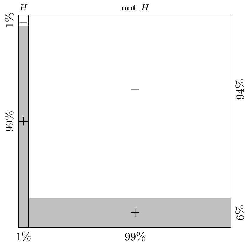
Figure 9.1: Intuition for Bayes’ Rule
The next video will give you deep insights about Bayes’ rule. You should be able to follow most of it, but you may want to come back to this video after trying some of the examples below.
9.3 Examples
The rare mineral unobtanium is present in only 1% of rocks in a mine. You have an unobtanium detector, which never fails to detect unobtanium when it is present. Otherwise, it is still reliable, returning accurate readings 90% of the time when unobtanium is not present.
- What is \(P(\text{unobtanium detected} | \text{unobtanium present})\)?
- What is \(P(\text{unobtanium present} | \text{unobtanium detected})\)?
(Hint: One of these probabilities can be read off directly from the question prompt. The other needs to be calculated using Bayes’ Rule.)
One application where Bayes’ Theorem has been extremely successful is spam filtering. From historical data, 80% of all e-mail is spam, and the phrase “free money” is used in 10% of spam e-mails. That is, \(P(\text{"free money"} | \text{spam}) = 0.1\). The phrase is also used in 1% of non-spam e-mails. A new e-mail has just arrived which contains the phrase “free money”. Given this information, what is the probability that it is spam, \(P(\text{spam} | \text{"free money"})\)?
A certain disease afflicts 10% of the population. A test for the disease is 90% accurate for patients with the disease and 80% accurate for patients without the disease. Suppose you test positive for the disease. What is the probability that you actually have the disease?