Lesson 49 Brownian Motion

The videos above discussed Brownian motion of particles moving in two or three dimensions; for simplicity, we will only consider Brownian motion in one dimension. This can be used to model, among other things, a particle moving along a line.

Shown below are 5 sample paths of Brownian motion.

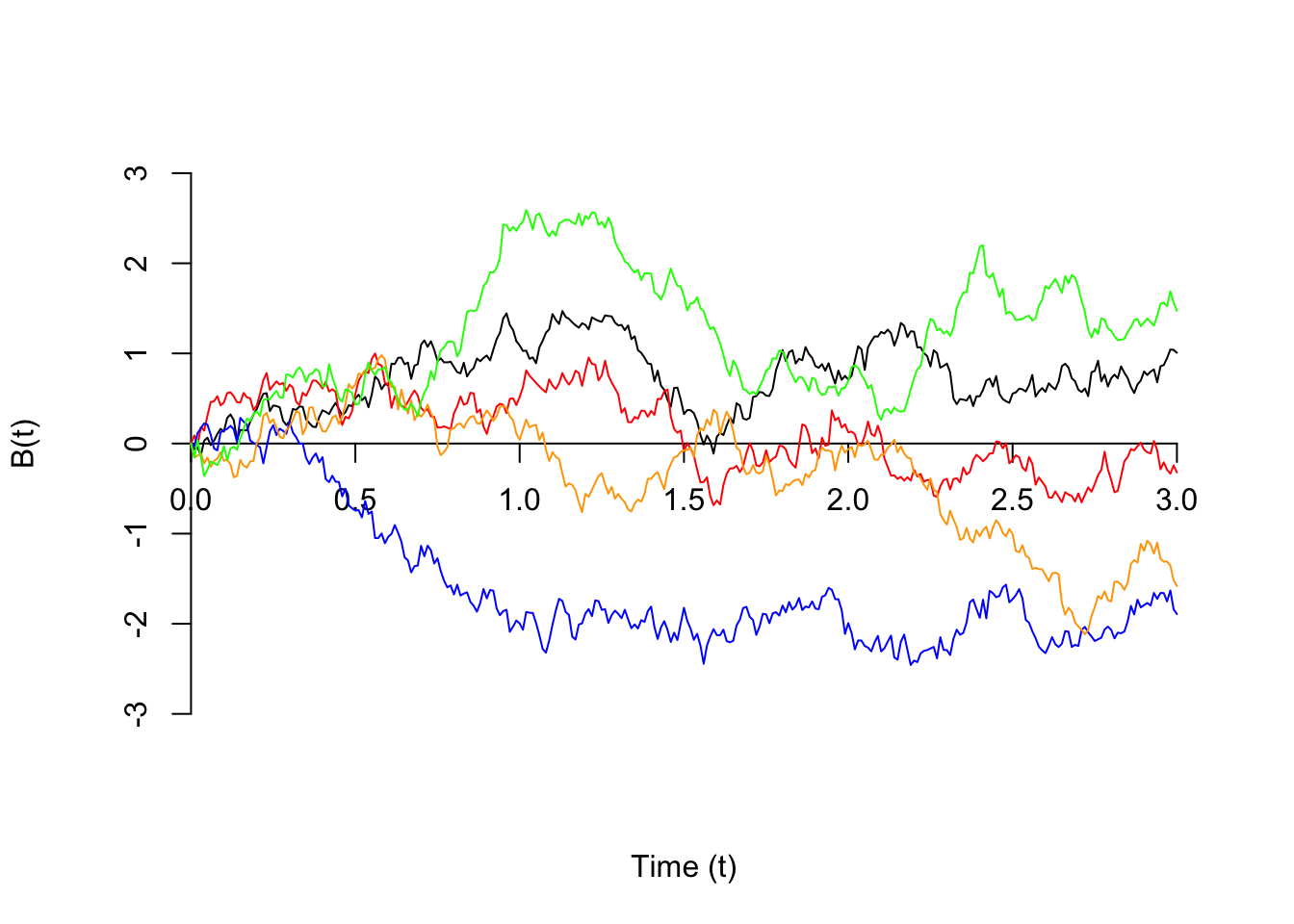
Definition 49.1 (Brownian Motion) Brownian motion $\{ B(t); t \geq 0 \}$ is a continuous-time process with the following properties:

The “particle” starts at the origin at $t=0$: $B(0) = 0$.
The displacement over any interval $(t_0, t_1)$, denoted by $B(t_1) - B(t_0)$, follows a $\text{Normal}(\mu=0, \sigma=\sqrt{\alpha(t_1 - t_0)})$ distribution.
Independent increments: The displacements over non-overlapping intervals are independent.

The parameter $\alpha$ controls the scale of Brownian motion.

These three properties allow us to calculate most probabilities of interest.

Example 49.1 (Motion of a Pollen Grain) The horizontal position of a grain of pollen suspended in water can be modeled by Brownian motion with scale $\alpha = 4 \text{mm}^2/\text{s}$.

What is the probability the pollen grain moves by more than 10 mm (in the horizontal direction) between 1 and 4 seconds?
If the particle is more than 5 mm away from the origin after 1 second, what is the probability the pollen grain moves by more than 10 mm between 1 and 4 seconds?

Solution. .

The displacement of the particle between 1 and 4 seconds is represented by $B(4) - B(1)$, which we know follows a $\text{Normal}(\mu=0, \sigma=\underbrace{\sqrt{4(4-1)}}_{\sqrt{12}})$ distribution.

Since the question does not indicate whether the displacement is positive or negative, we’re really interested in determining $P(|B(4) - B(1)| > 10)$. Because the distribution of $B(4) - B(1)$ is symmetric about $0$, this is the same as $2 P(B(4) - B(1) > 10)$ or $2 P(B(4) - B(1) < -10)$. \[\begin{align*} P(|B(4) - B(1)| > 10) &= 2 P(B(4) - B(1) > 10) \\ &= 2 P\big(\underbrace{\frac{B(4) - B(1) - 0}{\sqrt{12}}}_Z > \frac{10 - 0}{\sqrt{12}}\big) \\ &= 2 (1 - \Phi(\frac{10}{\sqrt{12}})) \\ &\approx .0039. \end{align*}\] b. The interval $(0, 1)$ does not overlap with the interval $(1, 4)$. Therefore, by the independent increments property, $B(1) = B(1) - B(0)$ is independent of $B(4) - B(1)$, and \[ P\Big(|B(4) - B(1)| > 10\ \big|\ |B(1)| > 5\Big) = P(|B(4) - B(1)| > 10) = .0039. \]

Brownian Motion as the Limit of a Random Walk

Brownian motion is the extension of a (discrete-time) random walk $\{ X[n]; n \geq 0 \}$ to a continuous-time process $\{ B(t); t \geq 0 \}$. The recipe is as follows:

Suppose the steps of the random walk happens at intervals of $\Delta t$ seconds. That is, \[ X(t) = X\left[\frac{t}{\Delta t}\right] \]
We let $\Delta t \to 0$. Since each step happens so quickly, it does not make sense to take steps of the same size. We should also rescale the size of the steps to be commensurate with how quickly they happen. The right rescaling is: \[ B(t) = \sqrt{\Delta t} X(t). \]

If we start with a discrete-time random walk and rescale time and step sizes in this way, we get Brownian motion. The animation below illustrates this.

Essential Practice

Brownian motion is used in finance to model short-term asset price fluctuation. Suppose the price (in dollars) of a barrel of crude oil varies according to a Brownian motion process; specifically, suppose the change in a barrel’s price $t$ days from now is modeled by Brownian motion $B(t)$ with $\alpha = .15$.
1. Find the probability that the price of a barrel of crude oil has changed by more than $1, in either direction, after 5 days.
2. Repeat (a) for a time interval of 10 days.
3. Given that the price has increased by $1 after one week (7 days), what is the probability that the price has increased by at least $2 after two weeks (14 days)?