Lesson 40 Normal Distribution
Motivation
The normal distribution is the most important distribution in all of probability and statistics. It is ubiquitous in the real world, as the above video demonstrates.
The normal distribution goes by a few other names:
- Gaussian distribution (especially common in engineering)
- the bell curve (in everyday life)
We will discuss the normal distribution in two stages:
- First, we will discuss the standard normal distribution.
- Then, we will discuss the general normal distribution, which has the same shape as the standard normal distribution, but with a different center and scale.
Standard Normal Distribution
Definition 40.1 (Standard Normal Distribution) A random variable \(Z\) is said to follow a standard normal distribution if its p.d.f. is \[\begin{equation} f(z) = \frac{1}{\sqrt{2\pi}} e^{-z^2 / 2}. \tag{40.1} \end{equation}\] The p.d.f. is non-zero for all real numbers \(-\infty < z < \infty\). It is conventional to use the letter \(Z\) for a standard normal random variable.
The c.d.f. of the standard normal distribution is \[\begin{equation} \Phi(x) \overset{\text{def}}{=} \int_{-\infty}^x f(t)\,dt. \tag{40.2} \end{equation}\] Note that it is conventional to use the Greek letter \(\Phi\) (“phi”) for the standard normal c.d.f., instead of \(F\). There is no closed-form formula for \(\Phi\), so we often leave our answers in terms of \(\Phi\). If a numerical value is required, we have a few options:
- We can use numerical integration.
- We can use software that calculates normal probabilities.
- We can use tables of the normal c.d.f., like this one.
The figure below shows the p.d.f. and c.d.f. of a standard normal distribution.
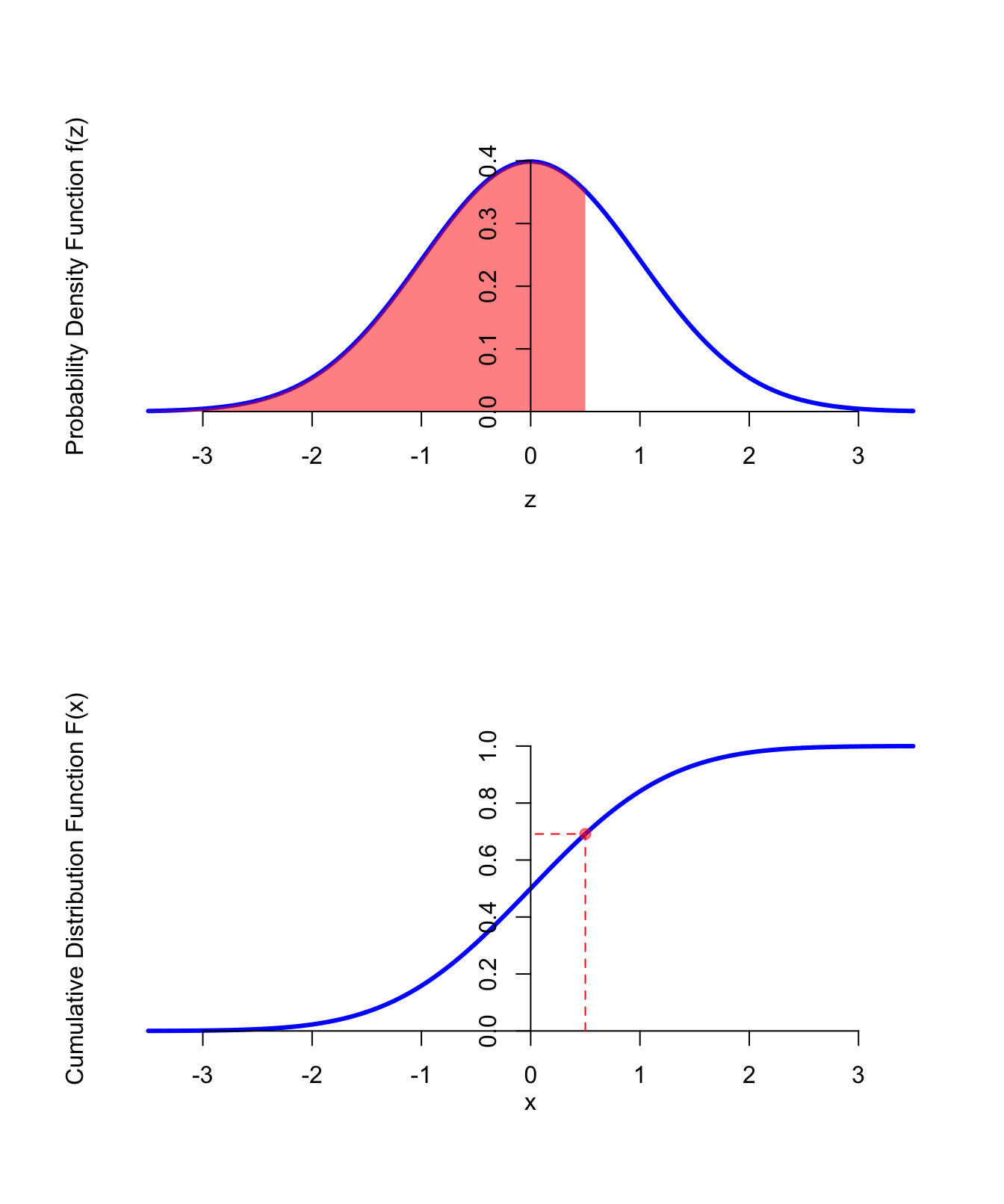
Figure 40.1: PDF and CDF of the Standard Normal Distribution
The Colab below shows how to use software to calculate probabilities involving a standard normal distribution.
Theorem 40.1 (Expected Value and Variance of the Standard Normal) Let \(Z\) be a standard normal random variable. Then: \[\begin{align*} E[Z] &= 0 & \text{Var}[Z] &= 1 \end{align*}\]
(General) Normal Distribution
Definition 40.2 (Normal Distribution) A random variable \(X\) is said to follow a \(\text{Normal}(\mu, \sigma)\) distribution if it can be expressed as \[\begin{equation} X = \mu + \sigma Z, \tag{40.3} \end{equation}\] where \(Z\) is a standard normal random variable.
Its p.d.f. is \[\begin{equation} f(x) = \frac{1}{\sigma\sqrt{2\pi}} e^{-( x - \mu)^2 / 2 \sigma^2}. \tag{40.4} \end{equation}\] To derive this, apply Theorems 36.1 and 36.2 to (40.1). However, we almost never use this p.d.f. for calculations. Instead, we typically use the representation (40.3) to convert the distribution to a standard normal before doing any calculations.
Note that the standard normal distribution is the \(\text{Normal}(\mu=0, \sigma=1)\) distribution.Shown below are the p.d.f.s and c.d.f.s of normal distributions for different values of \(\mu\) and \(\sigma\). Notice that \(\mu\) controls where the bell is centered, while \(\sigma\) controls how wide it is.
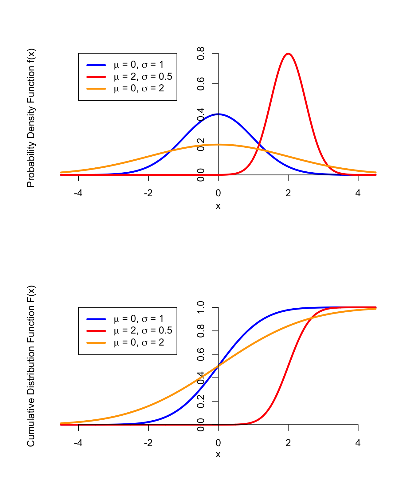
Figure 40.2: PDF and CDF of the Normal Distribution
The next theorem shows that \(\mu\) and \(\sigma\) can be interpreted as the center and spread, respectively.
By inverting (40.3), we see that \[\begin{equation} Z = \frac{X - \mu}{\sigma} \tag{40.5} \end{equation}\] follows a standard normal distribution. The process of converting a (general) normal random variable into a standard normal is known as standardization. One strategy for calculating probabilities from a normal distribution is to standardize and calculate the corresponding probability from the standard normal distribution.
The case study below shows how to calculate probabilities from a normal distribution, using a combination of algebra and software.
Essential Practice
Based on extensive data from an urban freeway near Toronto, Canada, “it is assumed that free speeds can best be represented by a normal distribution” (“Impact of Driver Compliance on the Safety and Operational Impacts of Freeway Variable Speed Limit Systems,” J. of Transp. Engr., 2011: 260–268). The mean and standard deviation reported in the article were 119 km/h and 13.1 km/h, respectively.
- What is the probability that the speed of a randomly selected vehicle is between 100 and 120 km/h?
- What speed characterizes the fastest 10% of all speeds?
- If five vehicles are randomly and independently selected, what is the probability that at least one car is traveling under the posted speed limit of 100 km/h?
Daily highs in San Luis Obispo in August are approximately normally distributed with a mean of \(76.9^\circ\textrm{F}\). The temperature exceeds 100 degrees Fahrenheit on about 1.5% of August days.
- What can you say about the standard deviation?
Suppose the mean increases by 2 degrees Fahrenheit. By what (multiplicative) factor will the percentage of 100-degree days increase?
(The moral of this exercise is: small changes in the mean can have massive effects on the tail probabilities.)
Suppose that the wrapper of a certain candy bar lists its weight as 2.13 ounces. Naturally, the weights of individual bars vary somewhat. Suppose that the actual weights of these candy bars vary according to a normal distribution with mean \(\mu = 2.20\) ounces and standard deviation \(\sigma = 0.04\) ounces.
- What proportion of candy bars weigh less than the advertised weight?
- If the weights of candy bars are independent, what is the expected number of candy bars before you encounter one that weighs less than the advertised weight?
- If the manufacturer decides that it’s unacceptable to have so many candy bars weigh less than the advertised weight, they might want to adjust the production process so that only 1 candy bar in 1000 weighs less than advertised. What should the mean of the actual weights be (assuming that the standard deviation of the weights remains 0.04 ounces)? Is this more or less than before? Why does this makes sense?
- If the manufacturer does not want to add weight to the candy bars (because this costs money), an alternative is to adjust the SD of the weights in the production process. If the mean weight remains at 2.20 ounces but only 1 candy bar in 1000 weighs less than the advertised weight, how small does the standard deviation of the weights need to be? Is this smaller or larger than before? Why does this makes sense?
Let \(Z\) be a standard normal random variable. Derive the p.d.f. of \(X = e^Z\). Sketch this p.d.f.
Hint: This is a transformation, so you can use the method of Lesson 36. When calculating the c.d.f., leave your answer in terms of \(\Phi\), the c.d.f. of the standard normal distribution. It does not have a closed-form expression, but you know its derivative. (What is the derivative of any c.d.f.?)
(This distribution has a name: the log-normal distribution. This is a popular distribution for modeling random variables with long right tails, such as income. Hopefully, you can appreciate this if you sketch the p.d.f.)