Lesson 12 Hypergeometric Distribution

Motivating Example

We revisit the Texas Hold’em example from Lesson 10, when we first learned about random variables. In that example, Alice was dealt

and she wanted to know the distribution of the number of diamonds among the community cards. If this random variable is at least 3, then she has a flush.

In Lesson 10, we derived the p.m.f. of the number of diamonds from scratch. In this lesson, we will derive the p.m.f. by matching this random variable to a template.

Theory

In probability, some distributions are so common that they have been given names. The first named distribution that we will learn is the hypergeometric distribution.

Theorem 12.1 (Hypergeometric Distribution) If a random variable can be described as the number of $\fbox{1}$s in $n$ random draws, without replacement, from the box \[ \overbrace{\underbrace{\fbox{0}\ \ldots \fbox{0}}_{N_0}\ \underbrace{\fbox{1}\ \ldots \fbox{1}}_{N_1}}^N, \] then its p.m.f. is given by \[\begin{equation} f(x) = \dfrac{\binom{N_1}{x}\binom{N_0}{n-x}}{\binom{N}{n}}, x=0, ..., n, \tag{12.1} \end{equation}\] where $N = N_1 + N_0$ is the number of tickets in the box.

We say that the random variable has a $\text{Hypergeometric}(n, N_1, N_0)$ distribution, and $n$, $N_1$, $N_0$ are called parameters of the distribution.

We will derive the formula (12.1) later in this lesson. First, let’s see how this result allows us to avoid most calculations.

Example 12.1 (The Number of Diamonds) In Alice’s case, the community cards are $5$ cards taken at random, without replacement, from a deck of $48$ cards. So we can represent it by a box model with $N=48$ tickets, with \[\begin{align*} \text{$N_1=11$ tickets labeled } \fbox{1} &\text{ representing the diamond cards} \\ \text{$N_0=37$ tickets labeled } \fbox{0} &\text{ representing the non-diamond cards}. \end{align*}\] Now, if we draw $n=5$ times from this box without replacement, then the number of $\fbox{1}$s we get corresponds to the number of diamonds.

Therefore, by Theorem 12.1, we know that the number of diamonds follows a $\text{Hypergeometric}(n=5, N_1=11, N_0=37)$ distribution. We can now write down the p.m.f. by plugging the values of the parameters $n$, $N_1$, $N_0$ into (12.1): \[ f(x) = \frac{\binom{11}{x} \binom{37}{5-x}}{\binom{48}{5}}, x=0, 1, \ldots, 5. \]

Now that we have a formula for the p.m.f., we can calculate probabilities by plugging numbers into it. So, for example, the probability that Alice gets a flush is: \[\begin{align*} P(X \geq 3) &= f(3) + f(4) + f(5) \\ &= \frac{\binom{11}{3} \binom{37}{5-3}}{\binom{48}{5}} + \frac{\binom{11}{4} \binom{37}{5-4}}{\binom{48}{5}} + \frac{\binom{11}{5} \binom{37}{5-5}}{\binom{48}{5}} \\ &\approx .0715. \end{align*}\]

Now, let’s derive the p.m.f. of the hypergeometric distribution. Understanding this derivation will help you remember the formula!

Proof (Theorem 12.1). If we number each ticket $1, 2, \ldots, N$, then there are $\binom{N}{n}$ equally likely unordered outcomes. Note that in this way of counting, the $\fbox{1}$s in the box are distinct. So drawing the first $\fbox{1}$ in the box is not the same as drawing the second $\fbox{1}$ in the box.

How many of the possible outcomes have exactly $x$ $\fbox{1}$s?

There are $\binom{N_1}{x}$ unordered ways to choose $x$ $\fbox{1}$s from the $N_1$ $\fbox{1}$s.
There are $\binom{N_0}{n-x}$ unordered ways to choose the remaining $n-x$ $\fbox{0}$s.

Since any one of the $\binom{N_1}{x}$ ways of choosing the $\fbox{1}$s can be paired with any one of the $\binom{N_0}{n-x}$ ways of choosing the $\fbox{0}$s, the total number of ways to choose $n$ tickets, resulting in $x$ $\fbox{1}$s and $n-x$ $\fbox{0}$s, is \[ \binom{N_1}{x} \cdot \binom{N_0}{n-x}, \] by the multiplication principle of counting (Theorem 1.1).

Therefore, the probability of getting exactly $x$ $\fbox{1}$s in $n$ draws is: \[ f(x) = P(X = x) = \dfrac{\binom{N_1}{x}\binom{N_0}{n-x}}{\binom{N}{n}}. \]

Visualizing the Distribution

Let’s graph the hypergeometric distribution for different values of $n$, $N_1$, and $N_0$.

First, we hold the number of draws constant at $n=5$ and vary the composition of the box.

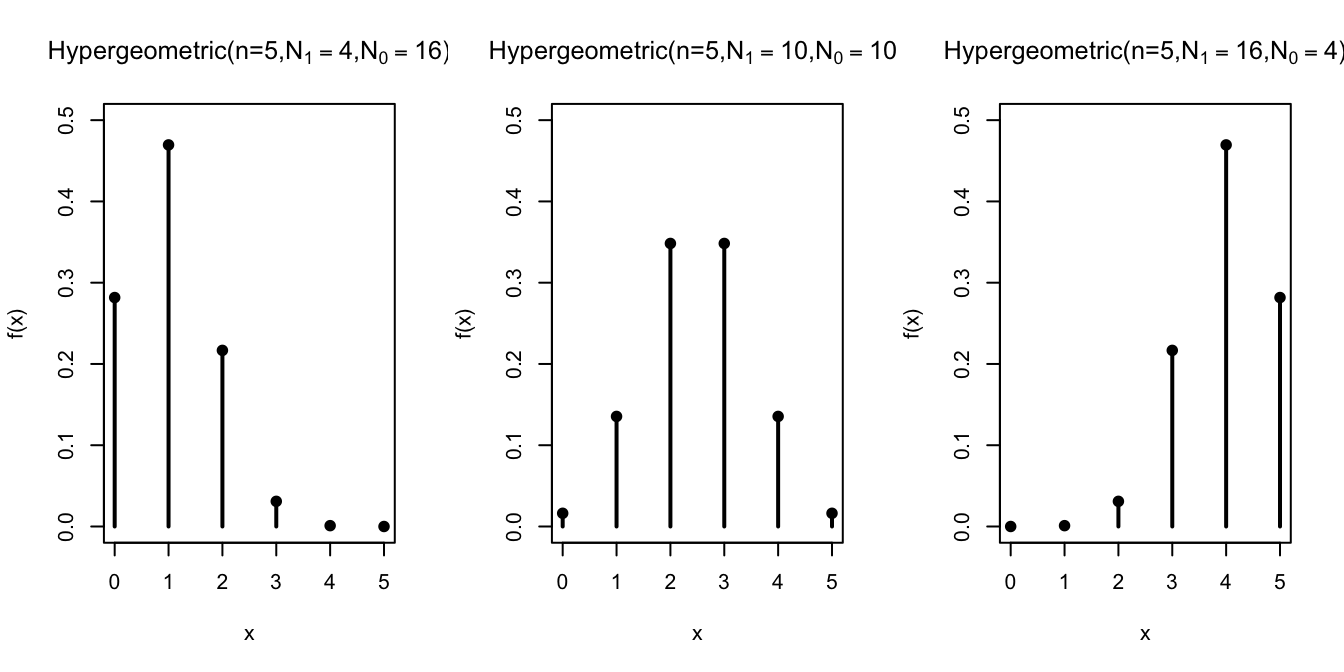
The distribution shifts, depending on the composition of the box. The more $\fbox{1}$s there are in the box, the more $\fbox{1}$s in the sample.

Next, we study how the distribution changes as a function of $n / N$, the relative fraction of tickets removed from the box. For all of the graphs below, $N_1 = N_0 = N/2$.

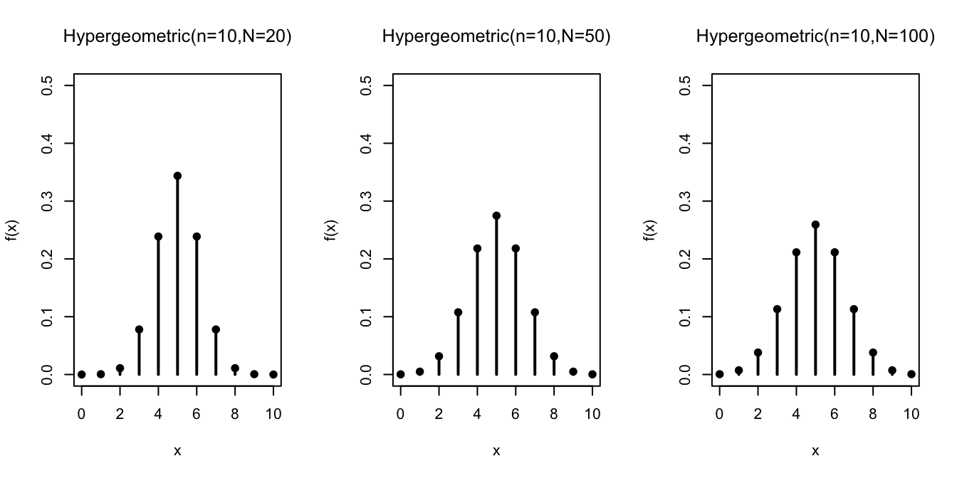
All three plots are symmetric, which makes sense, since there are exactly as many $\fbox{1}$s as $\fbox{0}$s in the box. However, when the number of draws makes up a large fraction of the box, as in the leftmost plot, the distribution is very tightly concentrated around intermediate values, such as 4, 5, and 6. This makes sense because sampling without replacement is “self-balancing”. Each time we draw a $\fbox{1}$, it becomes less likely that we will draw a $\fbox{1}$ again (and more likely to draw a $\fbox{0}$). This makes extreme outcomes, such as drawing all $\fbox{1}$s, less likely.

Calculating Hypergeometric Probabilities on the Computer

Calculating hypergeometric probabilities by hand is unwieldy when $n$, $N_1$, and $N_0$ are large. Fortunately, the hypergeometric distribution is built into many software packages.

For example, suppose we want to solve the following problem.

Example 12.2 (Capture-Recapture) One way to estimate the number of animals in a population is capture-recapture. For example, suppose we want to estimate the number of fish in a lake. Clearly, it is impractical to catch all of the fish. Instead, we capture $m$ fish one week, tag them, and release them back into the lake. We go back the next week, after these tagged fish have had a chance to mix with the population, and catch another $n$ distinct fish. Some, but not all, of these $n$ fish will be tagged. The number of tagged fish in this second catch allows us to estimate the population of fish in the lake.

Suppose there are actually 100 fish in the lake; we capture $m=20$ fish the first week and $n=30$ fish the next week. What is the probability that at least $7$ of the $30$ fish will be tagged?

Solution. We can represent this using a box model. The fish in the lake will be represented by $N=100$ tickets, with \[\begin{align*} \text{$N_1=20$ tickets labeled } \fbox{1} &\text{ representing the tagged fish} \\ \text{$N_0=80$ tickets labeled } \fbox{0} &\text{ representing the non-tagged fish}. \end{align*}\] Now, if we draw $n=30$ times from this box without replacement, then the number of $\fbox{1}$s we get corresponds to the number of tagged fish we get.

Therefore, the number of tagged fish is a $\text{Hypergeometric}(n=30, N_1=20, N_0=80)$ random variable. However, to calculate the probability that at least $7$ of the $30$ fish will be tagged, we have to evaluate the p.m.f. at 7, 8, 9, etc. This is a job for a computer, not a human.

In Python, we use a library called Symbulate. We first specify the parameters of the hypergeometric distribution; then we evaluate the p.m.f. using the .pmf() method. Note that .pmf() accepts either a single number or a list of numbers. If a list of numbers is passed into .pmf(), then it will evaluate the p.m.f. at each of those numbers, returning a list of probabilities.

from symbulate import *
probs = Hypergeometric(n=30, N1=20, N0=80).pmf(range(7, 31))
probs

## array([1.80287211e-01, 1.16176457e-01, 5.77600464e-02, 2.22376179e-02,
##        6.62820205e-03, 1.52341741e-03, 2.67853610e-04, 3.55743076e-05,
##        3.50270105e-06, 2.48771382e-07, 1.22310776e-08, 3.89715707e-10,
##        7.13438366e-12, 5.60558716e-14, 0.00000000e+00, 0.00000000e+00,
##        0.00000000e+00, 0.00000000e+00, 0.00000000e+00, 0.00000000e+00,
##        0.00000000e+00, 0.00000000e+00, 0.00000000e+00, 0.00000000e+00])

To add these probabilities, we call sum():

sum(probs)

## 0.38492014376629696

We could have also gotten the same answer by using c.d.f.s. Note that $P(X \geq 7) = 1 - F(6)$.

1 - Hypergeometric(n=30, N1=20, N0=80).cdf(6)

## 0.384920143766305

You can play around with the Python code in this Colab notebook.

It is possible to do the same calculation in R, a statistical programming language. Note that R uses different names for the parameters. Like Python, R can evaluate the p.m.f. at a single value or a vector of values.

probs <- dhyper(x=7:30, m=20, n=80, k=30)
probs

##  [1] 1.802872e-01 1.161765e-01 5.776005e-02 2.223762e-02 6.628202e-03
##  [6] 1.523417e-03 2.678536e-04 3.557431e-05 3.502701e-06 2.487714e-07
## [11] 1.223108e-08 3.897157e-10 7.134384e-12 5.605587e-14 0.000000e+00
## [16] 0.000000e+00 0.000000e+00 0.000000e+00 0.000000e+00 0.000000e+00
## [21] 0.000000e+00 0.000000e+00 0.000000e+00 0.000000e+00

To add these probabilities, we call sum():

sum(probs)

## [1] 0.3849201

We could have also gotten the same answer by using c.d.f.s. Notice how R uses the prefix d for p.m.f.s and the prefix p for c.d.f.s.

1 - phyper(6, m=20, n=80, k=30)

## [1] 0.3849201

You can play around with the R code in this Colab notebook.

Another Formula for the Hypergeometric Distribution (optional)

There is another formula for the hypergeometric p.m.f. that looks different but is equivalent to (12.1). It is based on counting the number of ordered outcomes, instead of the number of unordered outcomes. You should verify that this formula gives the same probabilities as (12.1).

Theorem 12.2 (Another Formula for the Hypergeometric) The p.m.f. of a $\text{Hypergeometric}(n, N_1, N_0)$ random variable can also be written as \[ f(x) = \frac{\binom{n}{x} \cdot \frac{N_1!}{(N_1 - x)!} \cdot \frac{N_0!}{(N_0 - n + x)!}}{\frac{N!}{(N-n)!}}. \]

Proof. There are $\frac{N!}{(N-n)!}$ ways to choose $n$ tickets from $N$, if we account for the order in which $n$ the tickets were drawn. How many of these ordered outcomes have exactly $x$ $\fbox{1}$s and $n-x$ $\fbox{0}$s?

Let’s start by counting the number of outcomes that look like \[\begin{equation} \underbrace{\fbox{1}, \ldots, \fbox{1}}_{x}, \underbrace{\fbox{0}, \ldots, \fbox{0}}_{n-x}, \tag{12.2} \end{equation}\] in this exact order. There are $N_1$ choices for the first $\fbox{1}$, $N_1 - 1$ choices for the second, and so on, until we get to the last $\fbox{1}$, for which there are $N_1 - x + 1$ choices. Then, there are $N_0$ choices for the first $\fbox{0}$, $N_0 - 1$ choices for the second, and so on. By the multiplication principle of counting (Theorem 1.1), there are \[\begin{equation} \underbrace{N_1 \cdot (N_1 - 1) \cdot \ldots \cdot (N_1 - x + 1)}_{\displaystyle\frac{N_1!}{(N_1 - x)!}} \cdot \underbrace{N_0 \cdot (N_0 - 1) \cdot \ldots \cdot (N_0 - (n - x) + 1)}_{\displaystyle\frac{N_0!}{(N_0 - n + x)!}}. \tag{12.3} \end{equation}\] ways to get an outcome like (12.2), in that exact order.

However, because we are counting ordered outcomes, we need to account for the possibility that the $\fbox{1}$s and $\fbox{0}$s were drawn in a different order than (12.2). There are $\binom{n}{x}$ ways to reorder the $\fbox{1}$s and $\fbox{0}$s, each of which can be obtained in (12.3) ways. So the total number of (ordered) ways to get $x$ $\fbox{1}$s and $n-x$ $\fbox{0}$s is \[ \binom{n}{x} \cdot \frac{N_1!}{(N_1 - x)!} \cdot \frac{N_0!}{(N_0 - n + x)!} \]

So the p.m.f. can be written as \[ f(x) = P(X = x) = \frac{\binom{n}{x} \cdot \frac{N_1!}{(N_1 - x)!} \cdot \frac{N_0!}{(N_0 - n + x)!}}{\frac{N!}{(N-n)!}}. \] It is easy to see that this formula is equivalent to (12.1), if you write out the binomial coefficients in (12.1) as factorials and regroup $\frac{n!}{x! (n-x)!}$ as $\binom{n}{x}$.

Essential Practice

Recall in the example from Lesson 10, there was another player, Bob, who had two Jacks and was looking to get a four-of-a-kind. For Bob, the random variable of interest was the number of Jacks among the community cards. Use a box model to argue that Bob’s random variable also has a hypergeometric distribution. What are its parameters?
In order to ensure safety, a random sample of cars on each production line are crash-tested before being released to the public. The process of crash testing destroys the car. Suppose that a production line contains 10 defective and 190 working cars. If 4 of these cars are chosen at random for crash-testing, what is:
1. the probability that at least 1 car will be found defective?
2. the probability that exactly 2 cars will be found defective?
The state proposes a lottery in which you select $6$ numbers from $1$ to $15$. When it is time to draw, the lottery selects $8$ different numbers, and you win if at least $4$ of the $6$ numbers you picked are among the $8$ numbers that the lottery drew. What is the probability you win the prize?

Additional Exercises

You are enrolled in $3$ courses this quarter, and the breakdown of majors by class is as follows:
- Class 1: $4$ Statistics majors and $6$ Computer Science majors
- Class 2: $17$ Statistics majors and $13$ Computer Science majors
- Class 3: $11$ Statistics majors and $9$ Computer Science majors
1. If you take a simple random sample of $20\%$ of the students in Class 1, what is the probability that the number of Statistics majors in your sample is equal to the number of Computer Science majors? (Note: In a simple random sample, each student can be selected at most once.)
2. Now, suppose you pick one of your $3$ classes at random and then choose a random sample of $20\%$ of students from that class. What is the probability that the number of Statistics majors in your sample is equal to the number of Computer Science majors in your sample?
In Texas Hold’em, each player has $2$ cards of their own, and all players share $5$ cards in the center of the table. A player has a flush when there are at least $5$ cards of the same suit out of the $7$ total cards. The deck is shuffled between hands, so that the probability you obtain a flush is independent from hand to hand. What is the probability that you get a flush at least once in $10$ hands of Texas Hold’em? (Hint: First, calculate the probability of a flush of spades. Then, repeat for the other suits, and add the probabilities together to obtain the overall probability of a flush.)
There are $25$ coins in a jar. $15$ are quarters, $7$ are dimes, and $3$ are pennies. Each time you reach in the jar, you are equally likely to pick any of the coins in the jar. The coins are not replaced in the jar after each draw. What is the minimum number of times you must reach in the jar to have at least a $50\%$ chance of getting all $3$ pennies? (Hint: In this question, $n$ is unknown. You will have to try a few different values of $n$ to get the answer.)