Lesson 28 Variance
Motivating Example
In Lesson 22, you showed that in roulette, every bet has exactly the same expected payoff. That is, their p.m.f.s have the same center of mass.
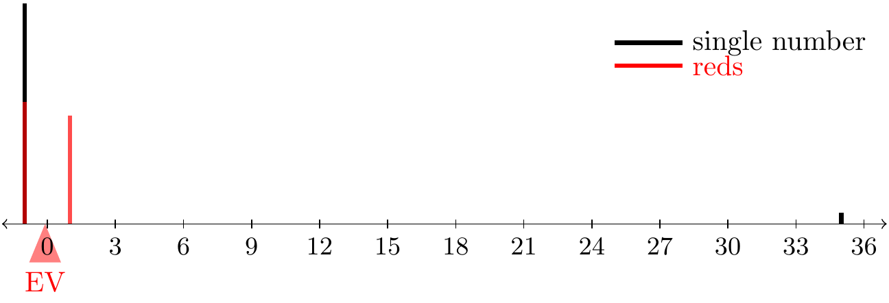
Does that mean that all bets are alike? No! A bet on a single number is riskier because you have a small chance (\(1/38\)) of making a lot of money ($35). A bet on reds, on the other hand, is smaller risk and smaller reward. How do we quantify how “risky” a bet is?
Theory
The expected value summarizes the center of a random variable. However, we have seen that two random variables can have the same center but very different distributions.
We also need to know how “spread out” the distribution is. The variance measures the “spread” of a distribution around its center.
In general, the variance (28.1) has to be computed using LOTUS.
Example 28.1 (Roulette Variances) The payout from a bet on a single number, \(X\), has p.m.f. \[ \begin{array}{r|cc} x & -1 & 35 \\ \hline f(x) & 37/38 & 1/38 \end{array}. \] We have already seen that \(E[X] = -\frac{2}{38}\). Its variance is: \[\begin{align*} \text{Var}[X] &= E[(X - -\frac{2}{38})^2] & \text{(plug in known value of $E[X]$)} \\ &= (35 - -\frac{2}{38})^2 \cdot \frac{1}{38} + (-1 - -\frac{2}{38})^2 \cdot \frac{37}{38} & \text{(LOTUS)}\\ &= 33.21 \end{align*}\]
The payout from a bet on a single number, \(Y\), has p.m.f. \[ \begin{array}{r|cc} y & -1 & 1 \\ \hline f(y) & 20/38 & 18/38 \end{array}. \] We have already seen that \(E[Y] = -\frac{2}{38}\). Its variance is: \[\begin{align*} \text{Var}[Y] &= E[(Y - -\frac{2}{38})^2] & \text{(plug in known value of $E[Y]$)} \\ &= (1 - -\frac{2}{38})^2 \cdot \frac{18}{38} + (-1 - -\frac{2}{38})^2 \cdot \frac{20}{38} & \text{(LOTUS)}\\ &= 0.997. \end{align*}\]
We see that the variances of these bets are very different, even though their expected values are the same.You might be surprised that the variance of a bet on a single number is so large. This is because variance is in squared units. That is, the variance of a bet on a single number is 33.21 dollars squared. Because squared units are often uninterpretable (what exactly is a “squared dollar”?), it is customary to report the square root of the variance, a number called the standard deviation.
For calculations, it is often easier to use the following “shortcut formula” for the variance.
Here is an example where we use the shortcut formula.
Example 28.3 (Variance of a Binomial Random Variable) The p.m.f. for a binomial random variable \(X\) is \[ f(x) = \binom{n}{x} \frac{N_1^x N_0^{n-x}}{N^n}, x=0, 1, \ldots, n. \] To calculate \(\text{Var}[X]\), we use the shortcut formula (28.2).
We already know \(E[X] = n\frac{N_1}{N}\), so we just need to calculate \(E[X^2]\). We showed that in Examples 24.3 and 26.4 that \[ E[X(X-1)] = n(n-1) \frac{N_1^2}{N_0^2}. \] Since \(E[X(X-1)] = E[X^2 - X] = E[X^2] - E[X]\), we can solve for \(E[X^2]\): \[\begin{align*} E[X^2] &= E[X(X-1)] + E[X] \\ &= n(n-1) \frac{N_1^2}{N_0^2} + n\frac{N_1}{N} \end{align*}\]
Now, we apply the shortcut formula (28.2): \[\begin{align*} \text{Var}[X] &= E[X^2] - E[X]^2 \\ &= n(n-1) \frac{N_1^2}{N_0^2} + n\frac{N_1}{N} - \left( n\frac{N_1}{N} \right)^2 \\ &= n \frac{N_1}{N} \left( (n-1) \frac{N_1}{N} + 1 - n \frac{N_1}{N} \right) \\ &= n \frac{N_1}{N} \underbrace{\left( 1 - \frac{N_1}{N} \right)}_{\frac{N_0}{N}}. \end{align*}\]
Later in this book, we will see an easier way to derive this same result.Now, if we know that a random variable \(X\) has a binomial distribution, we can use the formula \[ \text{Var}[X] = n\frac{N_1}{N} \frac{N_0}{N} \] instead of calculating it from scratch. We can derive formulas for the variances of all of the named distributions in a similar way. The formulas are provided in Appendix A.1.
If your random variable follows one of these named distributions, then you can just look up its variance in Appendix A.1. This is another benefit of learning these named distributions!
Essential Practice
Show that the variance of a \(\text{Poisson}(\mu)\) random variable is \(\mu\). (In other words, I am asking you to derive the result in the table above.)
(Hint: In Lesson 24, you derived \(E[X(X-1)]\) for a Poisson random variable. Use that result, and follow Example 28.3 above.)
Describe a random variable \(X\) with \(\text{Var}[X] = 0\).
In the carnival game chuck-a-luck, three dice are rolled. You make a bet on a particular number (1, 2, 3, 4, 5, 6) showing up. The payout is 1 to 1 if that number shows on (exactly) one die, 2 to 1 if it shows on two dice, and 3 to 1 if it shows up on all three. (You lose your initial stake if your number does not show on any of the dice.) If you make a $1 bet on the number three, what is the standard deviation of your net winnings?
(Hint: You already calculated the expected value in Lesson 22. Use that, in conjunction with the shortcut formula (28.2).)
Packets arrive at a certain node on the university’s intranet at 10 packets per minute, on average. Assume packet arrivals meet the assumptions of a Poisson process. What is the standard deviation of the number of arrivals you expect to see over a 5-minute period?
Additional Practice
Show that the variance of a \(\text{Hypergeometric}(n, N_1, N_0)\) random variable is \(n \frac{N_1}{N} \frac{N_0}{N} \frac{N-n}{N-1}\).
(Hint: You calculated \(E[X(X-1)]\) for a hypergeometric random variable in Lesson 24.)
Show that the variance of a \(\text{NegativeBinomial}(r, p)\) random variable is \(\frac{r(1-p)}{p^2}\).
(Hint: You calculated \(E[(X+1)X]\) for a negative binomial random variable in Lesson 24.)