Lesson 20 Conditional Distributions

Motivating Example

Continuing with the example from Lessons 18 and 19, suppose Xavier and Yolanda meet up later for coffee. Xavier has forgotten how many bets he won at roulette, but Yolanda clearly remembers that she won 3 bets. What information does this give Xavier about how many bets he won?

First, if Yolanda won 3 bets, Xavier knows that he had to have won at least once, since Yolanda only made two more bets than he did. But he cannot be sure whether he won 1, 2, or 3 bets. All he can do is assign probabilities to these possible values based on the information he has been given.

Theory

Xavier wants to know the distribution of the random variable $X$, given the information in another random variable $Y$. This is called the conditional distribution of $X$ given $Y$.

Definition 20.1 (Conditional Distribution) The conditional p.m.f. of $X$ given $Y$ is defined as \[\begin{equation} f_{X|Y}(x|y) \overset{\text{def}}{=} P(X = x | Y = y) = \frac{f(x, y)}{f_Y(y)}. \tag{20.1} \end{equation}\]

Visually, we are taking a row of the joint p.m.f. table and dividing the values by the total of that row. The process is illustrated in Figure 20.1.

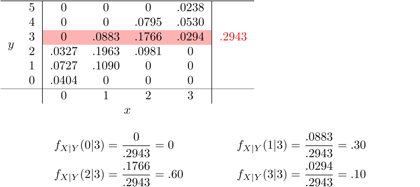
Figure 20.1: Calculating the Conditional Distribution of $Y$

Notice that the probabilities add up to $1.0$. This makes sense, since we have exhausted all the possible values that $X$ could be.

Figure 20.2 provides another view of what is going on when we divide by the marginal p.m.f. of $Y$. The probabilities in the joint p.m.f. $f(x, y)$ are correct relative to each other; the marginal p.m.f. $f_{Y}(y)$ is just a scaling factor to make the probabilities add up to $1.0$.

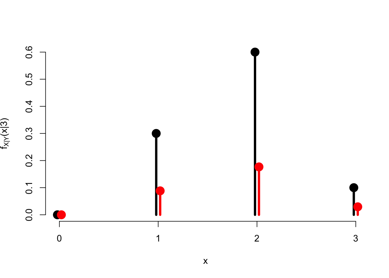
$The joint distribution $f(x, 3)$ in red vs. the conditional distribution $f_{X|Y}(x|3)$ in black$

Figure 20.2: The joint distribution $f(x, 3)$ in red vs. the conditional distribution $f_{X|Y}(x|3)$ in black

Let’s calculate another conditional distribution—this time using formulas, rather than tables.

Example 20.1 (Conditional Distributions of a Poisson Process) In San Luis Obispo, radioactive particles hit a Geiger counter according to a Poisson process at a rate of $\lambda = 0.8$ particles per second. Suppose that 7 particles are detected in the first 5 seconds. What is the distribution of the number of particles that are detected in the first 3 seconds?

Solution. If we let $X$ be the number of particles in the first 3 seconds and $Y$ be the number of particles in the first 5 seconds, then we are interested in the conditional distribution \[ f_{X|Y}(x | 7). \]

From (20.1), we know that this is \[ f_{X|Y}(x | 7) = \frac{f(x, 7)}{f_Y(7)}. \]

The marginal probability $f_Y(7)$ is easy to calculate. $Y$ is the number of arrivals on a $5$-second interval, which we know follows a $\text{Poisson}(\mu=5 \cdot 0.8)$ distribution, by Property 1 of a Poisson Process (see Lesson 17). Therefore: \[ f_Y(7) = e^{-5 \cdot 0.8} \frac{(5 \cdot 0.8)^7}{7!}. \]

To calculate the joint probability $f(x, 7)$, we first break the time interval $(0, 5)$ into two non-overlapping intervals, $(0, 3)$ and $(3, 5)$, as shown in Figure 20.3. We know from Property 2 of a Poisson Process (see Lesson 17) that the numbers of arrivals on non-overlapping intervals are independent. Let’s represent the number of arrivals on $(3, 5)$ by $Z \overset{\text{def}}{=} Y - X$ so that $Z$ is independent of $X$.

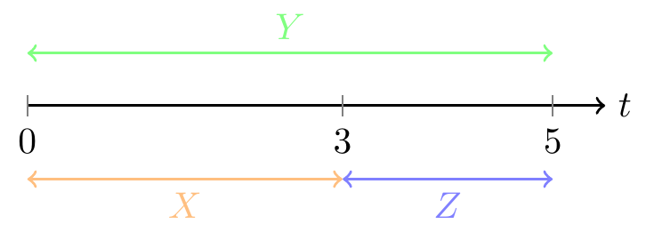
Figure 20.3: Breaking up a Poisson Process

Now, we calculate the joint probability: \[\begin{align*} f(x, 7) &= P(X=x \text{ and } Y=7) \\ &= P(X=x \text{ and } Z=7-x) \\ &= P(X=x) \cdot P(Z=7-x) & \text{(since $X$ and $Z$ are independent)} \\ &= e^{-(3 \cdot 0.8)} \frac{(3 \cdot 0.8)^x}{x!} \cdot e^{-(2 \cdot 0.8)} \frac{(2 \cdot 0.8)^{7-x}}{(7-x)!} \end{align*}\]

Putting everything together, we find that the conditional distribution is: \[\begin{align*} f_{X|Y}(x | 7) &= \frac{f(x, 7)}{f_Y(7)} \\ &= \frac{e^{-(3 \cdot 0.8)} \frac{(3 \cdot 0.8)^x}{x!} \cdot e^{-(2 \cdot 0.8)} \frac{(2 \cdot 0.8)^{7-x}}{(7-x)!}}{e^{-5 \cdot 0.8} \frac{(5 \cdot 0.8)^7}{7!}} \\ &= \frac{7!}{x! (7-x)!} \frac{(3 \cdot 0.8)^x \cdot (2 \cdot 0.8)^{7-x}}{(5 \cdot 0.8)^7} \\ &= \frac{\binom{7}{x} 3^x \cdot 2^{7-x}}{5^7} \end{align*}\]

This is just the p.m.f. of a $\text{Binomial}(n=7, N_1=3, N_0=2)$ distribution. The interpretation is this: given that there were 7 arrivals on the interval $(0, 5)$, each arrival has a $p=3/5$ chance of falling in the first 3 seconds, independently of the other arrivals.

Essential Practice

Let $X$ be the number of times a certain numerical control machine will malfunction on a given day. Let $Y$ be the number of times a technician is called on an emergency call. Their joint p.m.f. is given by \[ \begin{array}{rr|cccc} & 5 & 0 & .20 & .10 \\ y & 3 & .05 & .10 & .35 \\ & 1 & .05 & .05 & .10 \\ \hline & & 1 & 2 & 3\\ & & & x \end{array}. \]
1. Calculate the conditional distribution of $X$ given $Y=3$.
2. Calculate the conditional distribution of $Y$ given $X=2$.
3. Is $P(Y=3 | X=2)$ the same as $P(X=2 | Y=3)$?
Small aircraft arrive at San Luis Obispo airport according to a Poisson process at a rate of 6 per hour. What is the probability that (exactly) 5 small aircraft arrived in the first hour, given that (exactly) 12 aircraft arrived in the first two hours? First calculate an appropriate conditional distribution; then, use this conditional distribution to answer the question.
A fair coin is tossed 10 times. Let $X$ be the total number of heads in the 10 tosses. Let $Y$ be the number of heads in the first 6 tosses. Find the conditional distribution of $Y$, given $X = 7$. This is a named distribution we have learned. Which is it? Specify all parameters of this distribution.

(Hint: In order to identify the named distribution, it is easier to work with formulas rather than tables.)

Additional Exercises

Use the joint p.m.f. of the smaller and the larger of two dice rolls that you calculated in Lesson 18 to find the conditional distribution of the smaller number, given that the larger number was $4$.