C Fourier Transforms
Continuous-Time Fourier Transforms
The Fourier transform is an alternative representation of a signal. It describes the frequency content of the signal. It is defined as \[\begin{equation} G(f) \overset{\text{def}}{=} \int_{-\infty}^\infty g(t)e^{-j2\pi f t}\,dt. \tag{C.1} \end{equation}\] Notice that it is a function of frequency \(f\), rather than time \(t\). Notice also that it is complex-valued, since its definition involves the imaginary number \(j \overset{\text{def}}{=} \sqrt{-1}\).
The following video explains the visual intuition behind the Fourier transform. Note that this video uses \(i\) to denote the imaginary number \(\sqrt{-1}\), whereas we use \(j\) (which is common in electrical engineering, to avoid confusion with current).
To calculate the Fourier transform of a signal, we will rarely use (C.1). Instead, we will look up the Fourier transform of the signal in a table like Appendix D.1 and use properties of the Fourier transform (as shown in Appendix D.3).
Solution. This signal is most similar to \(e^{-t} u(t)\) in Appendix D.1, whose Fourier transform is \(\frac{1}{1 + j2\pi f}\). The only differences are:
- Our signal has an extra factor of 80 in front. This factor comes along for the ride by linearity of the Fourier transform.
- Our signal is time-scaled by a factor of 20, so we have to apply the scaling property. Since we multiplied by 20 in the time domain, we have to divide by 20 in the frequency domain, on both the inside and the outside.
Putting everything together, we see that the Fourier transform is: \[ G(f) = 80 \frac{1}{20} \frac{1}{1 + j 2\pi \frac{f}{20}}. \]
This is a complex-valued function. That is, at each frequency \(f\), \(G(f)\) is a complex number, with a real and an imaginary component. To make it easier to visualize, we calculate its magnitude using Theorem B.1. \[\begin{align*} |G(f)| = \sqrt{|G(f)|^2} &= \sqrt{G(f) \cdot G^*(f)} \\ &= \sqrt{\frac{4}{1 + j2\pi \frac{f}{20}} \cdot \frac{4}{1 - j2\pi \frac{f}{20}}} \\ &= \sqrt{\frac{4}{1 + (2\pi \frac{f}{20})^2}} \end{align*}\]
Now, the magnitude of the Fourier transform is a function we can easily visualize. From the graph, we see that the signal has more low-frequency content than high-frequency content.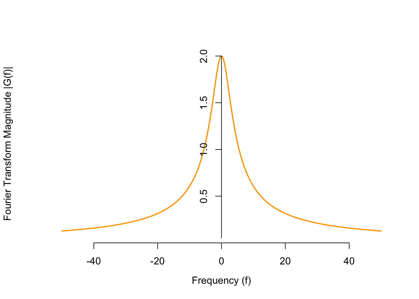
Discrete-Time Fourier Transforms
Discrete-time signals are obtained by sampling a continuous-time signal at regular time intervals. The sampling rate \(f_s\) (in Hz) specifies the number of samples per second. The signal below is sampled at a rate of \(f_s = 16\) Hz.
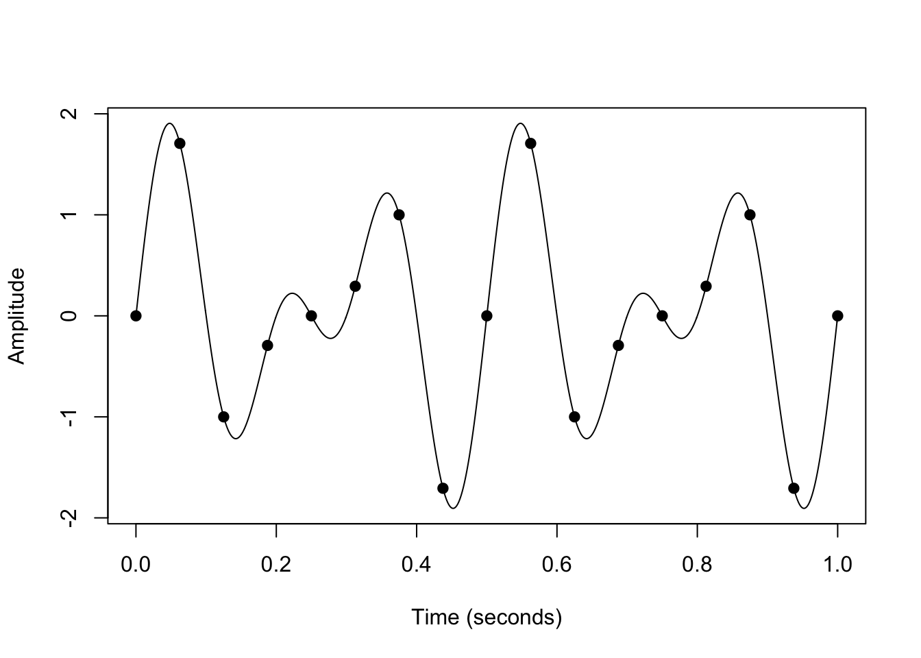
We write \(x[n] = x(t_n)\) for the \(n\)th time sample, where \(t_n = \frac{n}{f_s}\).
It’s possible to choose a sampling rate \(f_s\) that is too low. In the graph below, the underlying continuous-time signal (in black) is a sinusoid with a frequency of 14 Hz. However, because the discrete-time signal (in red) was sampled at a rate of 16 Hz, the sinusoid appears to have a frequency of 2 Hz.
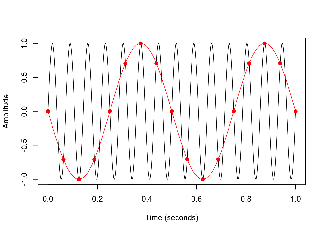
We say that the higher frequency is aliased by the lower one.
At a sampling rate of \(f_s\), any frequencies outside the range \[ (-f_s / 2, f_s / 2) \] will be aliased by a frequency inside this range. This “maximum frequency” of \(f_s / 2\) is known as the Nyquist limit.
Therefore, the Fourier transform of a discrete-time signal is effectively only defined for frequencies from \(-f_s/2\) to \(f_s/2\). Contrast this with the Fourier transform of a continuous-time signal, which is defined on all frequencies from \(-\infty\) to \(\infty\).
Aliasing is not just a theoretical problem. For example, if helicopter blades are spinning too fast for the frame rate of a video, then they can look like they are not spinning at all!
When calculating the Fourier transform of a discrete-time signal, we typically work with normalized frequencies. That is, the frequencies are in units of “cycles per sample” instead of “cycles per second”. (Another way to think about this is that we assume all discrete-time signals are sampled at 1 Hz.) As a result, the Nyquist limit is \(1/2\), so the Discrete-Time Fourier Transform is defined only for \(|f| < 0.5\).
\[\begin{align} G(f) &\overset{\text{def}}{=} \sum_{n=-\infty}^\infty g[n] e^{-j2\pi f t}\,dt & -0.5 < f < 0.5 \tag{C.2} \end{align}\]
To calculate the Fourier transform of a signal, we will rarely use (C.2). Instead, we will look up the Fourier transform of the signal in a table like Appendix D.2 and use properties of the Fourier transform (as shown in Appendix D.3).
Essential Practice
Calculate the Fourier transform \(G(f)\) of the continuous-time signal \[ g(t) = \begin{cases} 1/3 & 0 < t < 3 \\ 0 & \text{otherwise} \end{cases}. \] Graph its magnitude \(|G(f)|\) as a function of frequency.
Calculate the Fourier transform \(G(f)\) of the discrete-time signal \[ g[n] = \delta[n] + 0.4 \delta[n-1] + 0.4 \delta[n+1]. \] Graph \(G(f)\). (The Fourier transform should be a real-valued function, so you do not need to take its magnitude.)
Which of the following terms fill in the blank? The Fourier transform \(G(f)\) of a real-valued time signal \(g(t)\) is necessarily ….
- real-valued: \(G(f) \in \mathbb{R}\)
- positive-valued: \(G(f) > 0\)
- symmetric: \(G(-f) = G(f)\)
- conjugate symmetric: \(G(-f) = G^*(f)\)
(Hint: Write out \(G(f)\) and \(G(-f)\) according to the definition (C.1), and use Euler’s identity (Theorem B.2). Simplify as much as possible, using the facts that \(\cos(-\theta) = \cos(\theta)\) and \(\sin(-\theta) = -\sin(\theta)\).)
Which of the following terms fill in the blank? The Fourier transform \(G(f)\) of a real-valued and symmetric time signal \(g(t)\) is necessarily ….
- real-valued: \(G(f) \in \mathbb{R}\)
- positive-valued: \(G(f) > 0\)
- symmetric: \(G(-f) = G(f)\)
- conjugate symmetric: \(G(-f) = G^*(f)\)