Lesson 30 Properties of Covariance

Optional Video

This is an old video of mine. I’m including it in case it is helpful, but you do not need to watch it.

Theory

Calculating variance and covariance, even from the shortcut formulas (28.2) and (29.2), is tedious. Just as linearity simplified the calculation of expected values, the properties we learn in this lesson will simplify the calculation of variances and covariances.

Theorem 30.1 (Properties of Covariance) Let $X, Y, Z$ be random variables, and let $c$ be a constant. Then:

1. Covariance-Variance Relationship: $\displaystyle\text{Var}[X] = \text{Cov}[X, X]$ (This was also Theorem 29.1.)

2. Pulling Out Constants:

   $\displaystyle\text{Cov}[cX, Y] = c \cdot \text{Cov}[X, Y]$

   $\displaystyle\text{Cov}[X, cY] = c \cdot \text{Cov}[X, Y]$

3. Distributive Property:

   $\displaystyle\text{Cov}[X + Y, Z] = \text{Cov}[X, Z] + \text{Cov}[Y, Z]$

   $\displaystyle\text{Cov}[X, Y + Z] = \text{Cov}[X, Y] + \text{Cov}[X, Z]$

4. Symmetry: $\displaystyle\text{Cov}[X, Y] = \text{Cov}[Y, X]$
5. Constants cannot covary: $\displaystyle\text{Cov}[X, c] = 0$.

These properties follow immediately from the definition of covariance (29.1), so we omit their proofs.

Example 30.1 How does the variance change, when we multiply the random variable by a constant $a$? We answer this question using properties of covariance: $$\begin{align*} \text{Var}[aX] &= \text{Cov}[aX, aX] & \text{(Covariance-Variance Relationship)} \\ &= a \cdot a \cdot \text{Cov}[X, X] & \text{(Pulling Out Constants)} \\ &= a^2 \text{Var}[X] & \text{(Covariance-Variance Relationship)} \end{align*}$$

It makes sense that the variance should scale by $a^2$, since the variance is in squared units.

By combining the properties, we can derive new properties.

Example 30.2 Let $X, Y, Z, W$ be random variables. Then, by applying the distributive property twice: $$\begin{align*} \text{Cov}[X + Y, Z + W] &= \text{Cov}[X, Z+W] + \text{Cov}[Y, Z+W] \\ &= \text{Cov}[X, Z] + \text{Cov}[X, W] + \text{Cov}[Y, Z] + \text{Cov}[Y, W] \end{align*}$$

The result should remind you of FOILing from your high school algebra class, i.e., $$(x + y)(z + w) = xz + xw + yz + yw.$$ That is because multiplication also has a “distributive property”, just like covariance.

Here is a cute application of the properties of covariance that emphasizes the point that two variables can have zero covariance without being independent.

Example 30.3 (Covariance between the Sum and the Difference) Two fair six-sided dice are rolled. Let $X$ be the number on the first die. Let $Y$ be the number on the second die.

If $S = X + Y$ is their sum and $D = X - Y$ is their difference, what is $\text{Cov}[S, D]$?

$$\begin{align*} \text{Cov}[S, D] &= \text{Cov}[X + Y, X - Y] \\ &= \text{Cov}[X, X] + \text{Cov}[X, -Y] + \text{Cov}[Y, X] + \text{Cov}[Y, -Y] \\ &= \text{Var}[X]\ \ \ \ \ - \text{Cov}[X, Y]\ \ \ \ + \text{Cov}[X, Y] - \text{Var}[Y] \\ &= \text{Var}[X] - \text{Var}[Y] \\ &= 0. \end{align*}$$ In the second-to-last line, we used the fact that $X$ and $Y$ both represent the outcome when
a fair, six-sided die is rolled. So they must have the same distribution and the same variance. You could calculate $\text{Var}[X]$ and $\text{Var}[Y]$ if you’d like (they turn out to be about 2.917), but it is not necessary in this example because we know they will cancel.

Even though their covariance is zero, $S$ and $D$ are not independent! Think about it: if we are given that the sum was $S = 12$, we must have rolled two ⚅s. In other words, we know $D = 0$. Since one random variable gives us information about the other, they are not independent.

Here is yet another illustration of the power of these properties, to derive the formula for the variance of the binomial distribution. Compare the simplicity of this derivation with Example 28.3.

Example 30.4 (Variance of the Binomial Distribution) In Example 26.3, we argued that a $\text{Binomial}(n, N_1, N_0)$ random variable $X$ could be broken down as the sum of simpler random variables: $$X = Y_1 + Y_2 + \ldots + Y_n,$$ where $Y_i$ represents the outcome of the $i$th draw from the box. Since the draws are made with replacement, the $Y_i$s are independent.

The distribution of each $Y_i$ is $$\begin{array}{r|cc} y & 0 & 1 \\ \hline f(y) & \frac{N_0}{N} & \frac{N_1}{N} \end{array}.$$ It is not hard to calculate that $E[Y_i] = \frac{N_1}{N}$ and $$\begin{align*} \text{Var}[Y_i] &= E[Y_i^2] - E[Y_i]^2 \\ &= \left(0^2 \cdot \frac{N_0}{N} + 1^2 \cdot \frac{N_1}{N}\right) - \left(\frac{N_1}{N} \right)^2 \\ &= \frac{N_1}{N} \frac{N_0}{N}. \end{align*}$$

Now, we will use properties of covariance to express $\text{Var}[X]$ in terms of $\text{Var}[Y_i]$, which we calculated above: $$\begin{align*} \text{Var}[X] &= \text{Cov}[X, X] \\ &= \text{Cov}[Y_1 + Y_2 + \ldots + Y_n, Y_1 + Y_2 + \ldots Y_n] \\ &= \text{Cov}[Y_1, Y_1] + \text{Cov}[Y_1, Y_2] + \ldots + \text{Cov}[Y_n, Y_n] \end{align*}$$ Because the $Y_i$s are independent, all covariances of the form $\text{Cov}[Y_i, Y_j]$ for $i \neq j$ are zero. That leaves just terms of the form $\text{Cov}[Y_i, Y_i]$, which is equivalent to $\text{Var}[Y_i]$ by Property 1: $$\begin{align*} &= \text{Cov}[Y_1, Y_1] + \text{Cov}[Y_2, Y_2] + \ldots + \text{Cov}[Y_n, Y_n] \\ &= \text{Var}[Y_1] + \text{Var}[Y_2] + \ldots + \text{Var}[Y_n] \\ &= \frac{N_1}{N} \frac{N_0}{N} + \frac{N_1}{N} \frac{N_0}{N} + \ldots + \frac{N_1}{N} \frac{N_0}{N} \\ &= n \frac{N_1}{N} \frac{N_0}{N}. \end{align*}$$

This derivation gives insight into why the variance of a binomial distribution is $n \frac{N_1}{N} \frac{N_0}{N}$. The variance of each draw is $\frac{N_1}{N} \frac{N_0}{N}$, and the variance goes up by $n$ for the $n$ independent draws.

It is instructive to compare this derivation with the one for the hypergeometric distribution.

Example 30.5 (Variance of the Hypergeometric Distribution) In Example 26.3, we saw that a $\text{Hypergeometric}(n, N_1, N_0)$ random variable $X$ can be broken down in exactly the same way as a binomial random variable: $$X = Y_1 + Y_2 + \ldots + Y_n,$$ where $Y_i$ represents the outcome of the $i$th draw from the box. However, since the draws are made without replacement, the $Y_i$s are no longer independent. (Knowing that one draw was a $\fbox{1}$ makes it less likely for another draw to be a $\fbox{1}$.)

Each $Y_i$ still has expected value $E[Y_i] = \frac{N_1}{N}$ and variance $\text{Var}[Y_i] = \frac{N_1}{N} \frac{N_0}{N}$. But now we also need to consider the covariance between two different draws, since the draws are not independent. You calculated the covariance between two draws without replacement in Lesson 29. It is $\text{Cov}[Y_i, Y_j] = -\frac{1}{N-1} \frac{N_1}{N} \frac{N_0}{N}$.

Now, we will use properties of covariance to express $\text{Var}[X]$ in terms of $\text{Var}[Y_i]$ and $\text{Cov}[Y_i, Y_j]$, which we calculated above: $$\begin{align*} \text{Var}[X] &= \text{Cov}[X, X] \\ &= \text{Cov}[Y_1 + Y_2 + \ldots + Y_n, Y_1 + Y_2 + \ldots Y_n] \\ &= \text{Cov}[Y_1, Y_1] + \text{Cov}[Y_1, Y_2] + \ldots + \text{Cov}[Y_n, Y_n] \end{align*}$$ We have $n$ terms of the form $\text{Cov}[Y_i, Y_i] = \text{Var}[Y_i]$ and $n(n-1)$ terms of the form $\text{Cov}[Y_i, Y_j]$ for $i\neq j$. $$\begin{align*} &= n\text{Var}[Y_i] + n(n-1)\text{Cov}[Y_i, Y_j] \\ &= n \frac{N_1}{N} \frac{N_0}{N} - n(n-1) \frac{1}{N-1} \frac{N_1}{N} \frac{N_0}{N} \\ &= n \frac{N_1}{N} \frac{N_0}{N} \left(1 - \frac{n-1}{N-1}\right) \end{align*}$$

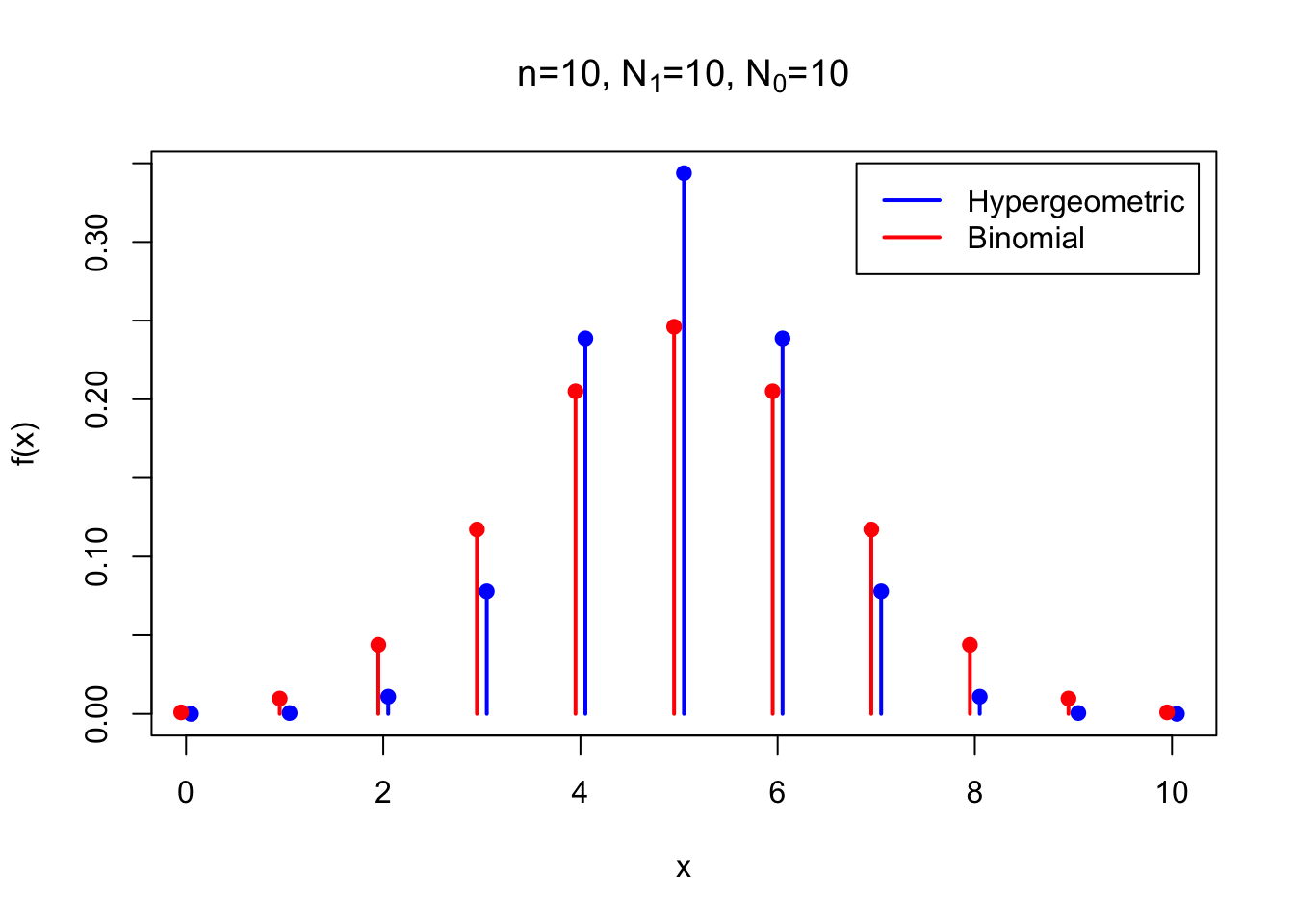
Notice that the variance of the hypergeometric is same as the variance of the corresponding binomial, except for the factor $\left(1 - \frac{n-1}{N-1}\right)$. This factor is less than 1, so the variance of the hypergeometric is always less than that of the corresponding binomial. This makes sense because the draws are made without replacement in the hypergeometric distribution. Each time we draw a $\fbox{1}$, we are less likely to draw a $\fbox{1}$ again (and more likely to draw a $\fbox{0}$). As a result, the number of $\fbox{1}$s is more likely to be somewhere near the middle in the hypergeometric distribution, so the variance will be smaller. The figure below compares the p.m.f.s of the two distributions.

The factor $\left(1 - \frac{n-1}{N-1}\right)$ is called the finite population correction. If our box had infinitely many tickets, then drawing without replacement is essentially the same as drawing with replacement. Thus, in the limit as $N \to \infty$, the hypergeometric distribution is the binomial distribution, and the finite population correction disappears. The finite population correction is only necessary because our boxes only contain a finite number of tickets.

Essential Practice

1. Let $W_1$ be your net winnings on a single spin of a roulette wheel when you bet $1 on a single number. This bet pays 35 to 1, meaning that for each dollar you bet, you win $35 if the ball lands on that number and lose $1 otherwise. We calculated the p.m.f., expected value, and variance of $W_1$ in Examples 22.1 and 28.1.

   Let $W_1, W_2, ..., W_{10}$ be independent random variables with the same distribution as $W_1$.

   Consider the random variables $X = 10 W_1$ and $Y = W_1 + W_2 + ... + W_{10}$. Which one represents…

   1. …your net winnings if you bet $1 on that number on each of 10 spins of the roulette wheel?
   2. …your net winnings if you bet $10 on that number on a single spin of the roulette wheel?

   Now, calculate $E[X]$, $E[Y]$, $\text{Var}[X]$, and $\text{Var}[Y]$. How do they compare?

2. Consider the following three scenarios:

   • A fair coin is tossed 3 times. $X$ is the number of heads and $Y$ is the number of tails.
   • A fair coin is tossed 4 times. $X$ is the number of heads in the first 3 tosses, $Y$ is the number of heads in the last 3 tosses.
   • A fair coin is tossed 6 times. $X$ is the number of heads in the first 3 tosses, $Y$ is the number of heads in the last 3 tosses.

   Use properties of covariance to calculate $\text{Cov}[X, Y]$ for each of these three scenarios. You should not need to use LOTUS or the shortcut formula for covariance.

   Hint 1: For the first scenario, write $Y$ as a function of $X$.

   Hint 2: For the second scenario, write $X = A + B$ and $Y = B + C$, where $A, B, C$ are independent random variables.

3. (This problem is challenging but rewarding.)

   A poker hand (5 cards) is dealt off the top of a well-shuffled deck of 52 cards. Let $X$ be the number of diamonds in the hand. Let $Y$ be the number of hearts in the hand.

   1. Do you think $\text{Cov}[X, Y]$ is positive, negative, or zero? Explain.
   2. Let $D_i (i=1, ..., 5)$ be a random variable that is $1$ if the $i$th card is a diamond and $0$ otherwise. What is $E[D_i]$?

   3. Let $H_i (i=1, ..., 5)$ be a random variable that is $1$ if the $i$th card is a heart and $0$ otherwise. Of course, $E[H_i]$ is the same as $E[D_i]$, since there are the same number of hearts as diamonds in a 52-card deck. What is $\text{Cov}[D_i, H_i]$? What is $\text{Cov}[D_i, H_j]$, when $i \neq j$? (Keep in mind that $D_i$ and $H_i$ are indicator random variables that only take on the values 0 or 1.)

      Hint: Make a table for the joint p.m.f. There are only 4 possible outcomes.

   4. Use your answers to parts b and c (and the properties of covariance, of course) to calculate $\text{Cov}[X, Y]$.

Additional Practice

1. Recall the coupon collector problem from Lesson 26:

   McDonald’s decides to give a Pokemon toy with every Happy Meal. Each time you buy a Happy Meal, you are equally likely to get any one of the 6 types of Pokemon. Let $X$ be the number of Happy Meals you have to buy until you “catch ’em all”.

   In that lesson, you calculated $E[X]$ using linearity of expectation. Now, use properties of covariance to calculate $\text{Var}[X]$.

2. At Diablo Canyon nuclear plant, radioactive particles hit a Geiger counter according to a Poisson process with a rate of 3.5 particles per second. Let $X$ be the number of particles detected in the first 2 seconds. Let $Z$ be the number of particles detected in the first 3 seconds. Find $\text{Cov}[X, Z]$.

   Hint: Note that $X$ and $Z$ are not independent. However, you should be able to write $Z = X + Y$, where $Y$ is a random variable that is independent of $X$.