Lesson 53 Stationary Processes
Motivation
What does it mean for a random process to remain the “same” over time? Obviously, the exact values will be different, since the process is random. The notion of a “stationary process” makes this notion precise.
Theory
Definition 53.1 (Stationary Process) A process \(\{ X(t) \}\) is called strict-sense stationary if the process is completely invariant under time shifts. That is, the distribution of \[ (X(t_1), X(t_2), ..., X(t_n)) \] matches the distribution of \[ (X(t_1 + \tau), X(t_2 + \tau), ..., X(t_n + \tau)) \] for any times \(t_1, ..., t_n\) and any time shift \(\tau\).
However, we will mostly be concerned with wide-sense stationary processes, which is less restrictive. A random process \(\{ X(t) \}\) is wide-sense stationary if its mean and autocovariance function are invariant under time shifts. That is:
- The mean function \(\mu_X(t)\) is constant. In this case, we will write the mean function as \(\mu_X(t) \equiv \mu_X\).
The autocovariance function \(C_X(s, t)\) only depends on \(s - t\), the difference between the times. In this case, we will write the autocovariance function as \(C_X(s, t) = C_X(s - t)\).
(For a discrete-time process, we require the autocovariance function \(C_X[m, n]\) to only depend on \(m - n\), and we write \(C_X[m, n] = C_X[m - n]\).)
Let’s determine whether some random processes are wide-sense stationary.
Example 53.1 (Random Amplitude Process) Consider the random amplitude process \[\begin{equation} X(t) = A\cos(2\pi f t) \tag{50.2} \end{equation}\] introduced in Example 48.1.
In Example 50.1, we showed that its mean function is \[ \mu_X(t) = 2.5 \cos(2\pi f t). \] This is not constant in \(t\), so this process cannot be wide-sense stationary. We do not even need to check the autocovariance function.
If we look at a graph of the process, it is clearly not stationary. If we shift the process by any amount that is less than a full period, then the process looks different. Shown on the graph below are 20 realizations of the original process \(\{ X(t) \}\) in blue, as well as 20 realizations of the time-shifted process \(\{ X(t - 0.3) \}\). The peaks and troughs are in different places.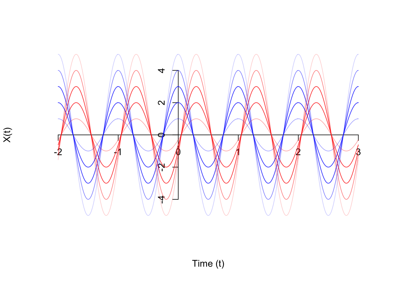
Example 53.2 (Poisson Process) Consider the Poisson process \(\{ N(t); t \geq 0 \}\) of rate \(\lambda\), defined in Example 47.1.
In Example 50.2, we showed that its mean function is \[ \mu_N(t) = \lambda t. \] This is not constant in \(t\), so we know that this process cannot be wide-sense stationary. We do not even need to check the autocovariance function.
Again, the fact that the Poisson process is not stationary is immediately apparent from a graph of the process. Shown below are 20 realizations of the original process \(\{ N(t) \}\) in blue, as well as 20 realizations of the time-shifted process \(\{ N(t - 1) \}\) in red. The time-shifted process may not even start at 0 at time 0!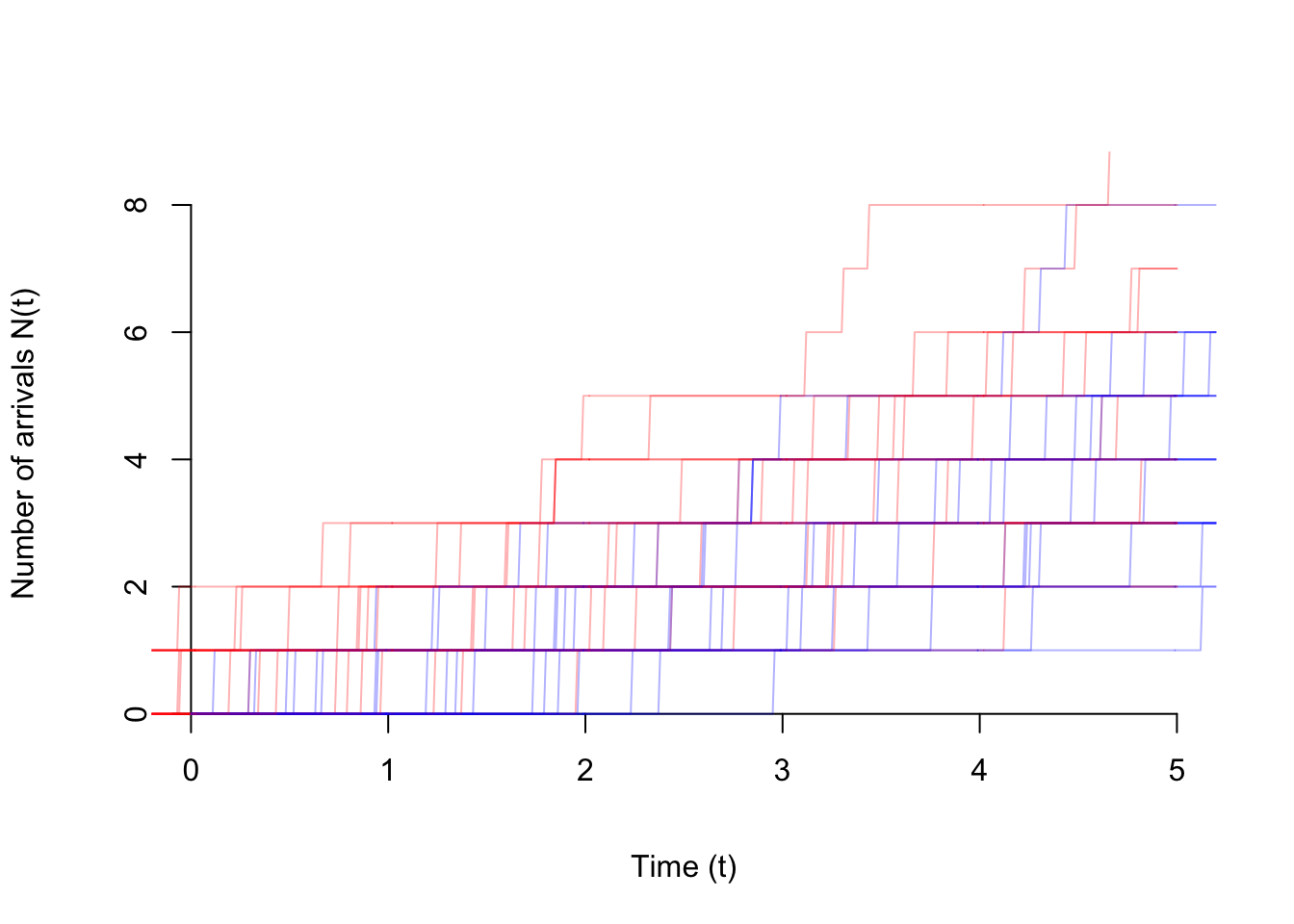
Example 53.3 (White Noise) Consider the white noise process \(\{ Z[n] \}\) defined in Example 47.2, which consists of i.i.d. random variables with mean \(\mu = E[Z[n]]\) and variance \(\sigma^2 \overset{\text{def}}{=} \text{Var}[Z[n]]\).
In Example 50.3, we showed that its mean function is \[ \mu_Z[n] \equiv \mu, \] which is constant, so the process could be wide-sense stationary. We need to check its autocovariance function.
In Example 52.3, we showed that its autocovariance function is \[ C_Z[m, n] = \begin{cases} \sigma^2 & m = n \\ 0 & m \neq n \end{cases}. \]
To see that this is a function of \(m - n\), we rewrite \(m = n\) as \(m - n = 0\): \[ C_Z[m, n] = \begin{cases} \sigma^2 & m - n = 0 \\ 0 & m - n \neq 0 \end{cases}. \]
This can be written more compactly using the discrete delta function \(\delta[k]\), defined as \[ \delta[k] \overset{def}{=} \begin{cases} 1 & k=0 \\ 0 & k \neq 0 \end{cases}. \] In terms of \(\delta[k]\), the autocovariance function is simply \[ C_Z[m, n] = \sigma^2 \delta[m - n]. \]
The graph below shows white noise \(\{ Z[n] \}\) in blue and time-shifted white noise \(\{ Z[n-1] \}\) in red. Visually, it is hard to tell the difference between the two, which is intutively why the process is stationary.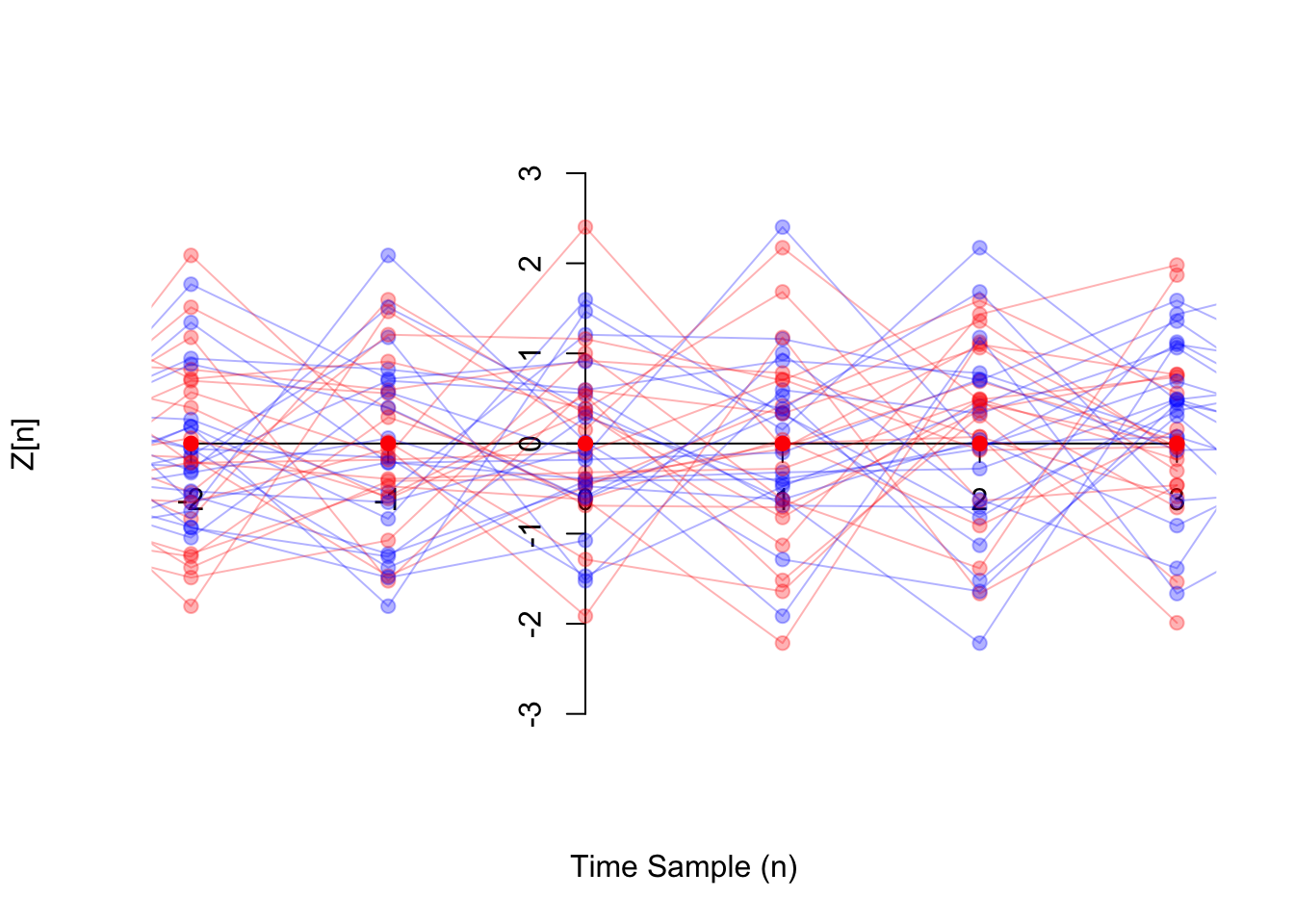
Example 53.4 (Random Walk) Consider the random walk process \(\{ X[n]; n\geq 0 \}\) from Example 47.3.
In Example 50.4, we calculated the mean function to be \[ \mu[n] = 0. \] This is constant, so the process might be wide-sense stationary. But we also need to check the autocovariance function.
In Example 52.4, we calculated the autocovariance function to be \[ C[m, n] = \min(m, n) \text{Var}[Z[1]]. \] This is not just a function of \(m - n\), so the process is not wide-sense stationary.
You might ask, “How can we be sure that there isn’t some way to manipulate \(\min(m, n)\) so that it is a function of \(m-n\)?” We can prove that it is impossible by testing a few pairs of values. For example, \((m, n) = (3, 2)\) and \((m, n) = (6, 5)\) are two pairs of values that are both separated in time by \(m - n = 1\) samples. If it were possible to reduce \(C[m, n]\) to a function \(C[m - n]\) of the difference only, then \(C[3, 2]\) would have to equal \(C[6, 5]\).
However, they are not equal: \(C[3, 2] = 2 \text{Var}[Z[1]]\), while \(C[6, 5] = 5 \text{Var}[Z[1]]\).Example 53.5 Let \(\{ X(t) \}\) be a continuous-time random process with
- \(E[X(t)] = 2\) for all \(t\), and
- \(\text{Cov}[X(s), X(t)] = 5e^{-3(s - t)^2}\) for all \(s\) and \(t\).
The mean function \(\mu_X(t) = E[X(t)]\) is constant and the autocovariance function \(C_X(s, t) = 5e^{-3(s - t)^2}\) is a function of \(\tau = s - t\) only, so the process is stationary.
Since the process is stationary, we can write the mean and autocovariance functions as \[\begin{align*} \mu_X &= 2 & C_X(\tau) &= 5e^{-3\tau^2}. \end{align*}\]Essential Practice
For these practice questions, you may want to refer to the mean and autocovariance functions you calculated in Lessons 50 and 52.
Consider a grain of pollen suspended in water, whose horizontal position can be modeled by Brownian motion \(\{B(t); t \geq 0\}\) with parameter \(\alpha=4 \text{mm}^2/\text{s}\), as in Example 49.1. Is \(\{ B(t); t \geq 0 \}\) wide-sense stationary?
Radioactive particles hit a Geiger counter according to a Poisson process at a rate of \(\lambda=0.8\) particles per second. Let \(\{ N(t); t \geq 0 \}\) represent this Poisson process.
Define the new process \(\{ D(t); t \geq 3 \}\) by \[ D(t) = N(t) - N(t - 3). \] This process represents the number of particles that hit the Geiger counter in the last 3 seconds. Is \(\{ D(t); t \geq 3 \}\) wide-sense stationary?
Consider the moving average process \(\{ X[n] \}\) of Example 48.2, defined by \[ X[n] = 0.5 Z[n] + 0.5 Z[n-1], \] where \(\{ Z[n] \}\) is a sequence of i.i.d. standard normal random variables. Is \(\{ X[n] \}\) wide-sense stationary?
(Hint: You can write \(m = n + 1\) as \(m - n = 1\).)
Let \(\Theta\) be a \(\text{Uniform}(a=-\pi, b=\pi)\) random variable, and let \(f\) be a constant. Define the random phase process \(\{ X(t) \}\) by \[ X(t) = \cos(2\pi f t + \Theta). \] Is \(\{ X(t) \}\) wide-sense stationary?