Lesson 10 Random Variables
Motivating Example
Texas hold ’em is a popular variant of poker. In Texas hold’em, each player starts with 2 cards (called “hole cards”) that are only known to them. In addition, there are 5 cards in the center (called “community cards”) that are shared by all the players. The player that wins is the one with the best five-card poker hand among the 7 cards (i.e., the 2 hole cards unique to them, plus the 5 community cards).
Alice and Bob are playing Texas hold’em using a single deck of cards. The 5 community cards have not been revealed yet.
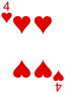
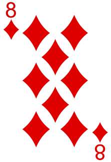
Alice is looking at her 2 hole cards, which are
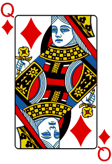
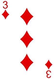
Because she already has two diamonds, she wonders how many more diamonds there are in the community cards. If there are 3 or more, then she has a flush.
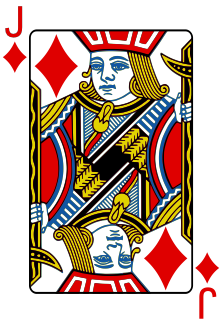
Bob, on the other hand, has the following hole cards
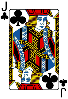
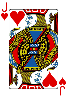
Because he has two jacks of different suits, he is less interested in the suit than in the number of jacks among the community cards. If there are 2, then he has a four-of-a-kind. If there are 0, then he just has a lowly pair.
Both Alice and Bob are interested in the same random phenomenon: the 5 community cards with their \(\binom{48}{5} \approx 1,712,304\) possible outcomes. However, their attention is drawn to different quantities:
- Alice to the number of diamonds
- Bob to the number of jacks
The number of diamonds and the number of jacks are two examples of random variables associated with this phenomenon. A random variable is simply a way of assigning a number to every possible outcome in a probability experiment. As we have seen, depending on the quantity of interest, there may be many random variables associated with the same probability experiment.
To appreciate that Alice and Bob are interested in different random variables, suppose the 5 community cards are revealed to be


Alice’s random variable (the number of diamonds) is 2, while Bob’s (the number of jacks) is 1. To help them decide how much to bet, Alice and Bob need to know the probabilities, such as
- the probability that the number of diamonds is at least 3.
- the probability that the number of jacks equals 2.
Theory
We describe random variables (such as the number of diamonds or the number of jacks) by the probabilities of their possible values. This is summarized by a function called the probability mass function.
Informally, the information contained in the p.m.f. is called the distribution of the random variable.
Example 10.1 (Calculating the P.M.F.) Let’s calculate the p.m.f. of the number of diamonds, \(X\), among the community cards. We deal 5 cards from a deck of cards that has had 4 cards removed (because they have already been dealt to Alice and Bob). Furthermore, we know that 2 of these cards were diamonds. So the deck has 48 cards left, of which 11 are diamonds.
First, we calculate \(f(0)\), the probability that \(X = 0\). In order for there to be no diamonds, all 5 cards must be selected from the \(48 - 11 = 37\) non-diamonds. So the probabiilty is \[ f(0) = P(X = 0) = \frac{\binom{37}{5}}{\binom{48}{5}} = .2546. \]
Next, we calculate \(f(1)\), the probability that \(X = 1\). We can choose any one of the 11 diamonds and pair it with any of the \(\binom{37}{4}\) ways to choose 4 cards from the non-diamonds. \[ f(1) = P(X = 1) = \frac{11 \cdot \binom{37}{4}}{\binom{48}{5}} = .4243. \]
Now, we calculate \(f(2)\), the probability that \(X = 2\). We can match any one of the \(\binom{11}{2}\) ways to choose 2 diamonds with the \(\binom{37}{3}\) ways to choose 3 non-diamonds: \[ f(2) = P(X = 2) = \frac{\binom{11}{2} \cdot \binom{37}{3}}{\binom{48}{5}} = .2496. \]
Continuing in this way, we can calculate \(f(3)\), \(f(4)\), and \(f(5)\). (Try these yourself!)
When the random variable only takes on a handful of possible values, we can write out the probabilities in a table.
| 0 | 1 | 2 | 3 | 4 | 5 | |
|---|---|---|---|---|---|---|
| \(f(x)\) | .2546 | .4243 | .2496 | .0642 | .0071 | .0002 |
Example 10.2 (Using the P.M.F.) In order for Alice to have a flush, there must be at least 3 diamonds among the community cards. Let’s see how she can easily calculate this probability, once she has the p.m.f. \(f(x)\).
In terms of the random variable \(X\), the probability that there are at least 3 diamonds is \(P(X \geq 3)\), which is \[\begin{align*} P(X \geq 3) &= f(3) + f(4) + f(5) \\ &= .0642 + .0071 + .0002 \\ &= .0715. \end{align*}\]
The complement rule (5.2) can sometimes save time. Although it would not helped in this example, we could have also calculated the probability as follows: \[\begin{align*} P(X \geq 3) &= 1 - P(X < 3) \\ &= 1 - (f(0) + f(1) + f(2)) \\ &= 1 - (.2546 + .4243 + .2496) \\ &= .0715. \end{align*}\]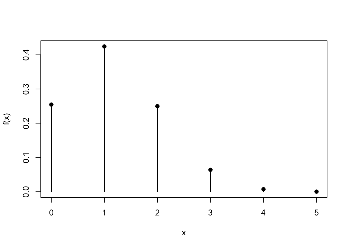
From the graph, it is immediately clear that 1 diamond is most probable. Unfortunately for Alice, it does not seem promising that she will get the 3 or more diamonds she needs to secure a flush.
Essential Practice
Continuing with the example from the lesson, let \(Y\) be the number of Jacks in the community cards. Calculate and graph the p.m.f. of \(Y\).
Two fair, six-sided dice are rolled.
- Let \(S\) be the sum of the two numbers. Calculate and graph the p.m.f. of \(S\).
- Let \(D\) be the absolute difference between the two numbers. (That is, \(D\) is always a positive number.) Calculate and graph the p.m.f. of \(D\).
A fair coin is tossed 5 times. Let \(Z\) be the number of heads. Calculate and graph the p.m.f. of \(Z\). Use the p.m.f. to calculate the probability of getting at least 2 heads.
Additional Exercises
- In college basketball, when a player is fouled while not in the act of shooting and the opposing team is “in the penalty,” the player is awarded a “1 and 1.” In the 1 and 1, the player is awarded one free throw, and if that free throw goes in, the player is awarded a second free throw. Find the p.m.f. of \(Y\), the number of points scored in a 1 and 1 given that any free throw goes in with probability \(0.7\), independent of any other free throw.