Lesson 51 Variance Function
Theory
Definition 51.1 (Variance Function) The variance function \(V(t)\) of a random process \(\{ X(t) \}\) is a function that specifies the variance of the process at each time \(t\). That is, \[ V(t) \overset{\text{def}}{=} \text{Var}[X(t)]. \]
For a discrete-time process, we notate the variance function as \[ V[n] \overset{\text{def}}{=} \text{Var}[X[n]]. \]The following video explains how to think about a variance function intuitively.
Let’s calculate the variance function of some random processes.
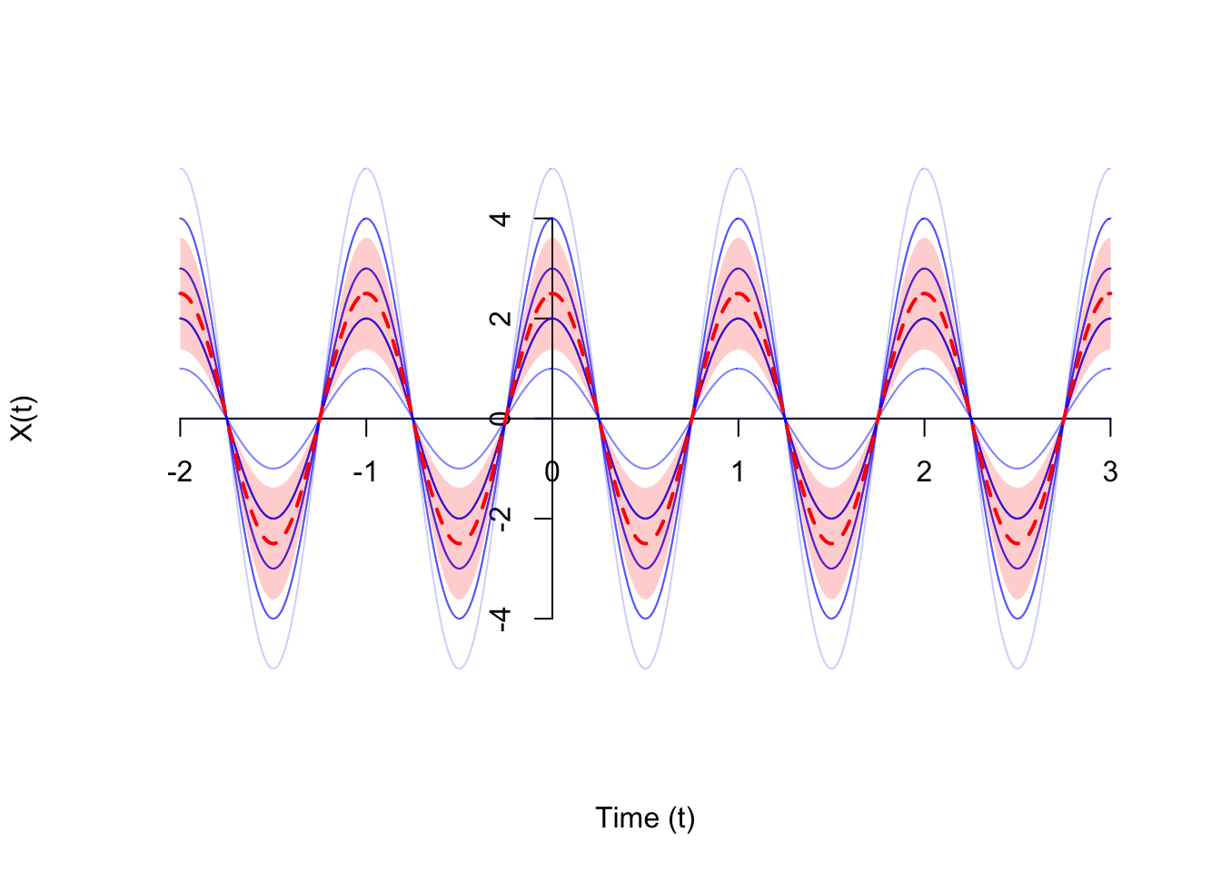
Example 51.1 (Random Amplitude Process) Consider the random amplitude process \[\begin{equation} X(t) = A\cos(2\pi f t) \tag{50.2} \end{equation}\] introduced in Example 48.1.
To be concrete, suppose \(A\) is a \(\text{Binomial}(n=5, p=0.5)\) random variable and \(f = 1\). To calculate the variance function, observe that the only thing that is random in (50.2) is \(A\). Everything else is a constant, so they can be pulled outside the variance. (However, we have to remember to square anything we pull outside the variance.) \[\begin{align*} V(t) = \text{Var}[X(t)] &= \text{Var}[A\cos(2\pi ft)] \\ &= \text{Var}[A] \cos^2(2\pi ft) \\ &= 1.25 \cos^2(2\pi ft), \end{align*}\] where in the last step, we used the formula for the variance of a binomial random variable, \(\text{Var}[A] = np(1-p) = 5 \cdot 0.5 \cdot (1 - 0.5) = 1.25\).Remember that the variance function \(V(t)\) measures the variability around the mean at time \(t\). Therefore, it makes sense to represent the variance function graphically as a band around the mean function. To construct this band, we do the following:
- Take the square root of the variance function so that it is in the same units as the mean function. (This is the same reason we defined the standard deviation as the square root of the variance.)
- Shade in a band of width \(\sqrt{V(t)}\) around the mean function \(\mu(t)\). That is, the band is lower-bounded by \(\mu(t) - \sqrt{V(t)}\) and upper-bounded by \(\mu(t) + \sqrt{V(t)}\).
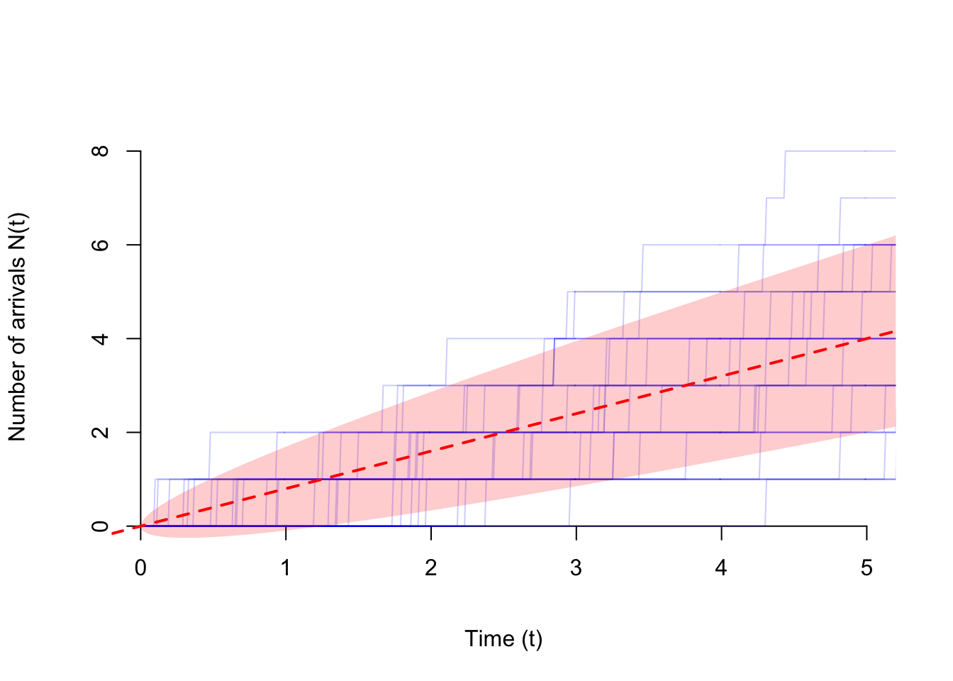
Example 51.2 (Poisson Process) Consider the Poisson process \(\{ N(t); t \geq 0 \}\) of rate \(\lambda\), defined in Example 47.1.
Recall that \(N(t)\) represents the number of arrivals on the interval \((0, t)\), which we know (by properties of the Poisson process) follows a \(\text{Poisson}(\mu=\lambda t)\) distribution. Since the variance of a \(\text{Poisson}(\mu)\) random variable is \(\mu\), we must have \[ V(t) = \text{Var}[N(t)] = \lambda t \]We represent the variance function of the Poisson process below as a band of width \(\sqrt{V(t)} = \sqrt{\lambda t}\) around the mean function \(\mu(t) = \lambda t\) (see Example 50.2).
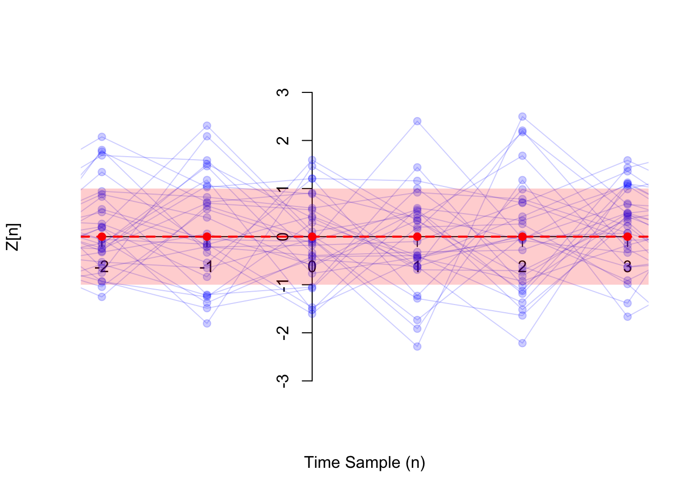
Shown below (in blue) are 30 realizations of a white noise process where the \(Z[n]\)s are i.i.d. standard normal so that \(\sigma^2 = 1\). The variance function of the white noise process is visualized below as a band of width \(\sqrt{V[n]} = 1\) around the mean function \(\mu[n] \equiv 0\) (see Example 50.3).
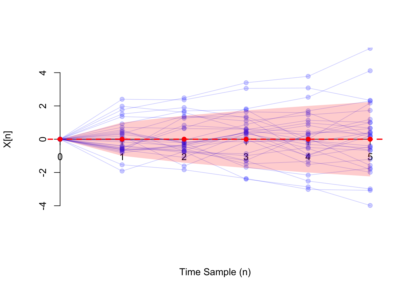
Shown below (in blue) are 30 realizations of the random walk process where the steps \(Z[n]\) are i.i.d. standard normal. In this case, the variance function (shown in red) is \(V[n] = n \cdot 1 \equiv n\). We visualize the variance function as a band of width \(\sqrt{V[n]} = \sqrt{n}\) around the mean function \(\mu[n] \equiv 0\) (see Example 50.4).
Essential Practice
Consider a grain of pollen suspended in water, whose horizontal position can be modeled by Brownian motion \(\{B(t)\}\) with parameter \(\alpha=4 \text{mm}^2/\text{s}\), as in Example 49.1. Calculate the variance function of \(\{ B(t) \}\).
Radioactive particles hit a Geiger counter according to a Poisson process at a rate of \(\lambda=0.8\) particles per second. Let \(\{ N(t); t \geq 0 \}\) represent this Poisson process.
Define the new process \(\{ D(t); t \geq 3 \}\) by \[ D(t) = N(t) - N(t - 3). \] This process represents the number of particles that hit the Geiger counter in the last 3 seconds. Calculate the variance function of \(\{ D(t); t \geq 3 \}\).
Consider the moving average process \(\{ X[n] \}\) of Example 48.2, defined by \[ X[n] = 0.5 Z[n] + 0.5 Z[n-1], \] where \(\{ Z[n] \}\) is a sequence of i.i.d. standard normal random variables. Calculate the variance function of \(\{ X[n] \}\).
Let \(\Theta\) be a \(\text{Uniform}(a=-\pi, b=\pi)\) random variable, and let \(f\) be a constant. Define the random phase process \(\{ X(t) \}\) by \[ X(t) = \cos(2\pi f t + \Theta). \] Calculate the variance function of \(\{ X(t) \}\). (Hint: LOTUS)