Lesson 33 Continuous Random Variables
Motivating Example
In a Poisson process, the number of arrivals in any interval is a random variable that follows a Poisson distribution. But what about the time of the first arrival? This is also a random variable, but of a different kind. The time of the first arrival does not have to be an integer. It can equal \(1.2\) seconds, \(2.173\) seconds, \(\sqrt{2}\) seconds, or even \(\pi\) seconds. In fact, any real number from \(0\) to \(\infty\) is a possible value of this random variable.
To be concrete, suppose radioactive particles hit a Geiger counter according to a Poisson process with a rate of \(\lambda = 0.8\) particles per second. We will represent the time of the first arrival—that is, the time that the first particle hits the Geiger counter—by \(T\). We can calculate probabilities involving \(T\). For example, we can calculate the probability that the first particle arrives after 2 seconds by rewriting this event in terms of the number of arrivals on an interval: \[ P(T > 2) = P(\text{0 particles between 0 and 2 seconds}) \] We know that the number of particles between 0 and 2 seconds follows a \(\text{Poisson}(\mu=0.8 \cdot 2)\) distribution, so we just need to evaluate the p.m.f. at \(x=0\): \[\begin{equation} P(T > 2) = e^{-0.8 \cdot 2} \frac{(0.8 \cdot 2)^0}{0!} = e^{-1.6} \approx .202. \tag{33.1} \end{equation}\]
We can also calculate the probability that the first arrival happens between \(2\) and \(3\) seconds, as: \[ P(2 < T < 3) = P(T > 2) - P(T > 3). \] We calculate \(P(T > 3)\) in much the same way as we calculated \(P(T > 2)\) above: \[\begin{equation} P(T > 3) = e^{-0.8 \cdot 3} \frac{(0.8 \cdot 3)^0}{0!} = e^{-2.4} \approx .091. \tag{33.2} \end{equation}\] So we see that \[ P(2 < T < 3) = e^{-1.6} - e^{-2.4} \approx .111. \]
Although we can calculate specific probabilities involving \(T\), how do we describe its distribution? In particular:
- What is its c.d.f.?
- Does it have a p.m.f.?
We will answer these questions in this lesson and more.
Theory
First, we calculate the c.d.f. of \(T\), which is straightforward from its definition (11.1).Example 33.1 (The CDF of the First Arrival) Remember that the c.d.f. is defined as \(F(t) = P(T \leq t)\) as a function of \(t\). First, we use the complement rule: \[ F(t) = P(T \leq t) = 1 - P(T > t). \] Now, we calculate \(P(T > t)\), in much the same way that we calculated \(P(T > 2)\) in (33.1) and \(P(T > 3)\) in (33.2): \[ P(T > t) = e^{- 0.8 \cdot t} \frac{(0.8 \cdot t)^0}{0!} = e^{-0.8 t}. \] This formula works for \(t \geq 0\). Since times are positive, we know that \[ P(T > t) = 1 \] for \(t < 0\).
Putting everything together, the c.d.f. of \(T\) is \[ F(t) = 1 - P(T > t) = \begin{cases} 1 - e^{-0.8 t} & t \geq 0 \\ 0 & t < 0 \end{cases}. \] This function is graphed below.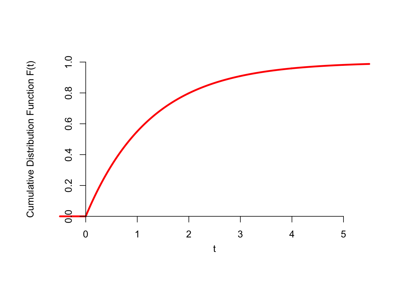
Figure 33.1: CDF of the First Arrival
Notice how different this c.d.f. is, compared with the ones we graphed in Lesson 11. In Figure 11.1, the c.d.f. was a step function, with a jump at each possible value of the random variable. By contrast, the c.d.f. above is continuous. This is the main distinction between the kinds of random variables we were studying before, which are called discrete random variables, and the kinds of random variables we study in this lesson, which are called continuous random variables.
With discrete random variables, we can visualize the shape of the distribution by graphing its p.m.f. Recall that the p.m.f. specified the probability that the random variable is equal to \(x\). Continuous random variables do not have a p.m.f. because the probability of any exact outcome is zero.
Example 33.2 (Probability of a Single Outcome) Continuing with Example 33.1, what is the probability that the first particle hits the Geiger counter at exactly 2 seconds—that is, \(P(T = 2.00000...)\)?
First, consider the probability that the first arrival is in the interval \((2 - \epsilon, 2 + \epsilon)\), where \(\epsilon\) is a small positive number. No matter how small an \(\epsilon\) we choose, this probability will always be greater than the probability that the first arrival happens at exactly 2 seconds, since this interval includes 2 seconds, as well as some other outcomes. (For example, if \(\epsilon = 0.05\), then this interval would also include the possibility that the first arrival happens at 1.98 seconds or 2.01 seconds.)
The number of arrivals on the interval \((2 - \epsilon, 2 + \epsilon)\) is a Poisson random variable with parameter \(\mu = 0.8 \cdot 2\epsilon\). Therefore, the probability that there are no arrivals on the interval is: \[\begin{align*} P(\text{at least 1 arrival on interval}) &= 1 - P(\text{no arrivals on interval}) \\ &= 1 - e^{-0.8 \cdot 2\epsilon} \frac{(0.8 \cdot 2 \epsilon)^0}{0!} \\ &= 1 - e^{-1.6 \epsilon}. \end{align*}\] But \(\epsilon\) can be arbitrarily small. As \(\epsilon \to 0\), this probability approaches 0.
Therefore, the probability that the first arrival happens at exactly 2 seconds is zero.Because the probability of every outcome in a continuous random variable is zero, continuous random variables cannot be described by their p.m.f. Instead, they are described by a similar function called the probability density function.
The following video presents an alternative perspective on the p.d.f. It gives more insight into what a “probability density” is. It also reinforces the message that \(P(X = x) = 0\) for any continuous random variable \(X\).
Example 33.3 (The PDF of the First Arrival) Continuing with Example 33.1, the c.d.f. was calculated to be \[ F(t) = \begin{cases} 1 - e^{-0.8 t} & t \geq 0 \\ 0 & t < 0 \end{cases}. \] Taking the derivative, we have \[\begin{equation} f(t) = F'(t) = \begin{cases} 0.8 e^{-0.8 t} & t \geq 0 \\ 0 & t < 0 \end{cases}. \tag{33.3} \end{equation}\] Figure 33.2 below shows the p.d.f., along with the c.d.f. Since the p.d.f. is the derivative of the c.d.f., it is the slope of the c.d.f. at a given value of \(t\). The steeper the c.d.f., the higher the p.d.f.
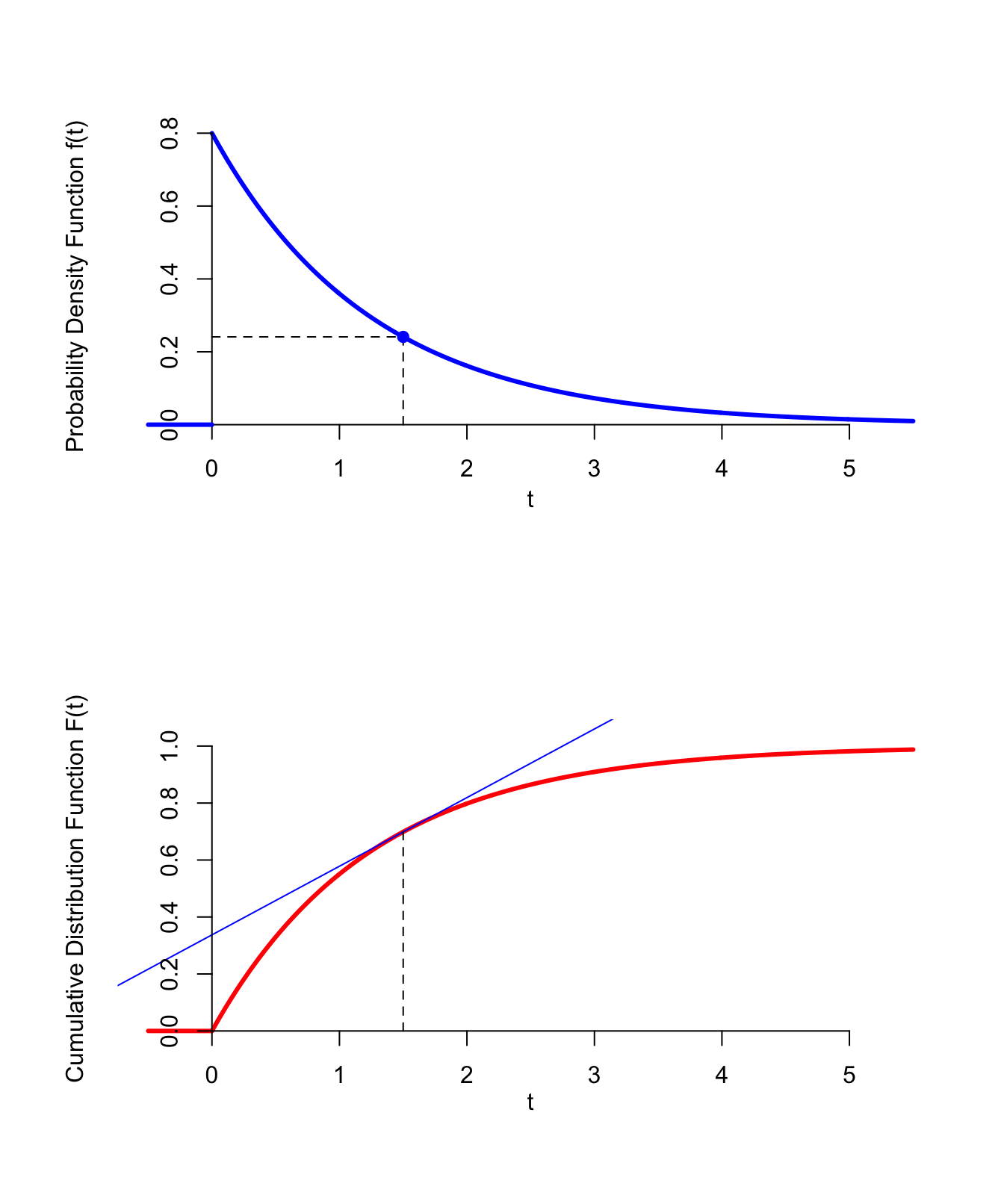
Figure 33.2: PDF from the CDF
This p.d.f. tells us that the first arrival is more likely to happen sooner, rather than later. However, the values of the p.d.f. are not easy to interpret. They do not represent probabilities, but rather probability densities.
If the values of the p.d.f. do not represent probabilities, how do we calculate probabilities using the p.d.f.? It turns out that areas under the p.d.f. represent probabilities.
Theorem 33.1 says that probabilities correspond to areas under the p.d.f. This is another way to see that the probability of any single outcome must be 0. The probability that \(X = x\) would be the integral from \(x\) to \(x\); since there is no area under the curve at \(x\), this probability must be 0.
Let’s recalculate the probabilities from the Motivating Example, now using the p.d.f. (33.3).
Example 33.4 (Calculating Probabilities Using the PDF) We know that the p.d.f. of the first arrival, \(T\), is \[ f(t) = \begin{cases} 0.8 e^{-0.8 t} & t \geq 0 \\ 0 & t < 0 \end{cases}. \] To calculate probabilities using Theorem 33.1, we integrate the p.d.f.
For example, the probability that the first arrival happens between 2 and 3 seconds is: \[ P(2 < T < 3) = \int_2^3 f(t)\,dt = \int_2^3 0.8 e^{-0.8 t}\,dt = .111, \] and the probability that the first arrival happens after 2 seconds is \[ P(T > 2) = \int_2^\infty f(t)\,dt = \int_2^\infty 0.8 e^{-0.8 t}\,dt = .202.\] The areas that these probabilities represent are shown on the graphs below.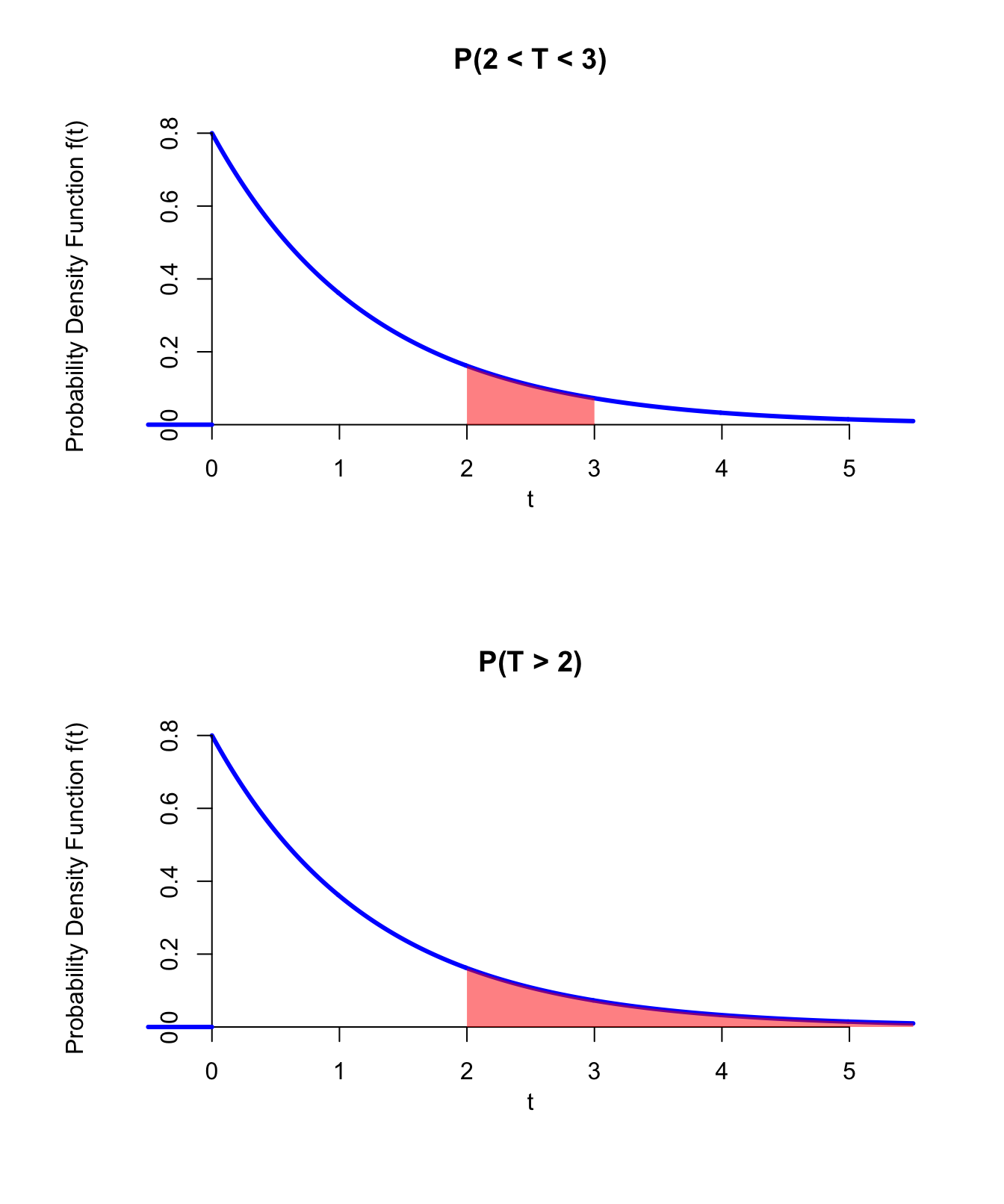
Figure 33.3: PDF of the First Arrival
What about the probability that the first arrival happens before 3 seconds? Technically, we should integrate the p.d.f. from \(-\infty\) to \(3\). However, \(f(t) = 0\) for \(-\infty < t < 0\), so we effectively integrate the p.d.f. from \(0\) to \(3\): \[ P(T < 3) = \int_{-\infty}^3 f(t)\,dt = \int_0^3 0.8 e^{-0.8 t}\,dt = .909. \]
So far, we saw that we take the derivative of the c.d.f. to get the p.d.f. We can also go in reverse: if we have the p.d.f., we can take its integral to get the c.d.f. \[\begin{equation} F(x) = \int_{-\infty}^x f(t)\,dt. \tag{33.4} \end{equation}\]
Example 33.5 ((Re)deriving the CDF of the First Arrival) Suppose we only knew the p.d.f. of the first arrival \(T\): \[ f(t) = \begin{cases} 0.8 e^{-0.8 t} & t \geq 0 \\ 0 & t < 0 \end{cases}. \]
To calculate the c.d.f. at \(x\), we integrate the p.d.f. up to \(x\). Since the p.d.f. is 0 when \(t < 0\), the integral effectively starts from \(t=0\). \[ F(x) = \int_{-\infty}^x f(t)\,dt = \int_0^x 0.8 e^{-0.8 t}\,dt = 1 - e^{-0.8 x}. \] (This integral can be calculated using the \(u\)-substitution \(u=-0.8 t\), or using Wolfram Alpha.)Figure 33.4 below illustrates how areas under the p.d.f. translate to values of the c.d.f.
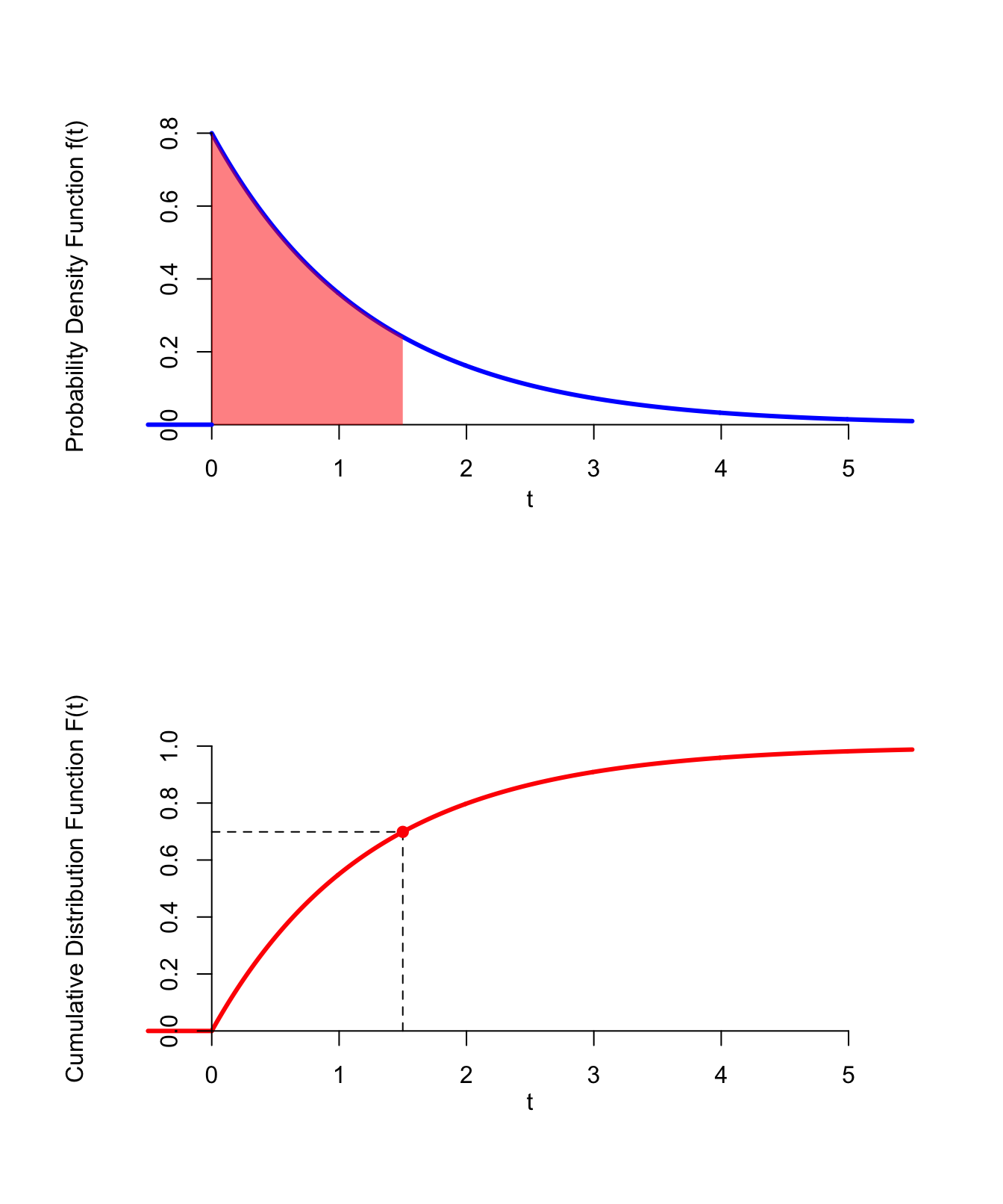
Figure 33.4: CDF from the PDF
Optional Video
This video (not my own) does an excellent job explaining the mechanics of calculations involving p.d.f.s and c.d.f.s. If you felt that you understood the material above well enough to do the Essential Practice below, you probably do not need to watch this video. Do not get too caught up in the calculus; remember that you can always use Wolfram Alpha to compute any integrals or derivatives.
Essential Practice
Packets arrive at a certain node on the university’s intranet at 10 packets per minute, on average. Assume packet arrivals meet the assumptions of a Poisson process.
- What is the p.d.f. of \(T\), the time of the first arrival?
- What is the probability that the first arrival happens between 10 seconds and 30 seconds? (Note that the rate in the problem is given in minutes.)
Two Cal Poly students, Ferris and Cameron, are frequently late to class. Cal Poly classes start at 10 minutes past the hour mark.
Let \(X\) be the time (in minutes) that Ferris arrives at class after the hour mark. The p.d.f. of \(X\) is \[ f_X(x) = \begin{cases} \frac{1}{60} & 0 \leq x < 60 \\ 0 & \text{otherwise} \end{cases}. \] Let \(Y\) be the time (in minutes) that Cameron arrives at class after the hour mark. The p.d.f. of \(Y\) is \[ f_Y(y) = \begin{cases} \frac{60 - y}{1800} & 0 \leq y < 60 \\ 0 & \text{otherwise} \end{cases}. \]
- Sketch a graph of the two p.d.f.s. Without doing any calculations, who is more likely to arrive on time (i.e., within the first 10 minutes of the hour)?
- Determine the c.d.f.s of \(X\) and \(Y\).
- Calculate the probability that Ferris arrives on time. You should be able to calculate this probability in three ways: (1) finding the area under the p.d.f. using geometry, (2) finding the area under the p.d.f. using calculus, and (3) using the c.d.f.
- Calculate the probability that Cameron arrives on time. You should also be able to calculate this probability in three ways.
The distance (in hundreds of miles) driven by a trucker in one day is a continuous random variable \(X\) whose cumulative distribution function (c.d.f.) is given by: \[ F(x) = \begin{cases} 0 & x < 0 \\ x^3 / 216 & 0 \leq x \leq 6 \\ 1 & x > 6 \end{cases}. \]
- Determine the p.d.f. Sketch a graph.
- Calculate the probability that the trucker travels more than 500 miles in a day. (You should be able to calculate this in at least 2 ways: directly from the c.d.f. and using the p.d.f. that you calculated in the previous part.)
- Calculate the probability that the trucker travels exactly 200 miles in a day.
Let \(T\) be how late that a professor lets her class out (in minutes). (If \(T\) is negative, then she finishes the class early.) The p.d.f. of \(T\) is \[ f(t) = \begin{cases} c(2 + t) & -2 < t < 0 \\ c(2 - t) & 0 \leq t < 2 \\ 0 & \text{otherwise} \end{cases}, \] where \(c\) is a constant.
- Determine the value of \(c\) necessary to make this a proper p.d.f. (Hint: What does the total probability have to be?) Sketch the p.d.f.
- Calculate the probability that the professor finishes between 1 minute early and 30 seconds late, i.e., \(P(-1 < T < 0.5)\).