Lesson 46 Central Limit Theorem

Motivation

In Lesson 45, we saw that calculating the exact distribution of a sum of i.i.d. random variables, $S_n = X_1 + X_2 + \ldots + X_n$ is a lot of work. Each time we add another random variable, we have to calculate a convolution, which requires calculating an integral. For arbitrary p.m.f.s and p.d.f.s, calculating many convolutions is impractical.

However, we often work with the sum of hundreds or even thousands of random variables. Since getting the exact distribution of $S_n$ is impractical, we need an approximation that is accurate and easy to use. The Central Limit Theorem provides that approximation.

Theory

Theorem 46.1 (Central Limit Theorem for Sums) Let $X_1, ..., X_n$ be independent and identically distributed (i.i.d.) random variables. Then, for $n$ large, their sum \[ S_n = X_1 + ... + X_n \] is approximately normally distributed.

Therefore, to calculate a probability such as $P(S_n \leq x)$, we can use a normal distribution. Of course, we need the parameters of the normal distribution. That is, we need to specify $\mu$ and $\sigma$. We choose these parameters to match the expectation $E[S_n]$ and the standard deviation $\text{SD}[S_n]$, which we can calculate using properties of expectation and covariance: \[\begin{align*} \mu = E[S_n] &= E[X_1 + X_2 + ... + X_n] \\ &= E[X_1] + E[X_2] + ... + E[X_n] & \text{(linearity of expectation)} \\ &= n E[X_1] & \text{($X_i$s are identically distributed)} \\ \sigma^2 = \text{Var}[S_n] &= \text{Cov}[S_n, S_n] \\ &= \text{Cov}[X_1 + ... + X_n, X_1 + ... + X_n] \\ &= \text{Cov}[X_1, X_1] + \text{Cov}[X_1, X_2] + ... + \text{Cov}[X_n, X_n] & \text{(properties of covariance)} \\ &= \text{Var}[X_1] + ... + \text{Var}[X_n] & \text{($X_i$s are independent)} \\ &= n\text{Var}[X_1] & \text{($X_i$s are identically distributed)} \\ \sigma = \sqrt{\sigma^2} &= \sqrt{n} \text{SD}[X_1]. \end{align*}\]

Since the mean of a list of numbers is just their sum divided by $n$, the mean of $n$ i.i.d. random variables is also approximately normal. (Scaling a normal random variable by a constant just produces another normal distribution.)

Theorem 46.2 (Central Limit Theorem for Means) Let $X_1, ..., X_n$ be independent and identically distributed (i.i.d.) random variables. Then, for $n$ large, their (sample) mean \[ \bar X_n = \frac{X_1 + ... + X_n}{n} \] is approximately normally distributed.

The parameters of this normal distribution are: \[\begin{align*} \mu = E[\bar X_n] &= E[\frac{S_n}{n}] \\ &= \frac{n E[X_1]}{n} \\ &= E[X_1] \\ \sigma^2 = \text{Var}[\bar X_n] &= \text{Var}[\frac{S_n}{n}] \\ &= \frac{1}{n^2} \text{Var}[S_n] \\ &= \frac{1}{n^2} n \text{Var}[X_1] \\ &= \frac{\text{Var}[X_1]}{n} \\ \sigma = \text{SD}[\bar X_n] &= \frac{\text{SD}[X_1]}{\sqrt{n}}. \end{align*}\]

The sample mean will hover around the expected value of each observation, and the uncertainty (as measured by the standard deviation) approaches 0 as $n \to \infty$. This is the same calculation that we did in Lesson 32 to prove the Law of Large Numbers, which says that the sample mean converges to this expected value as $n \to\infty$. For any finite number $n$, the sample mean will be close to, but not exactly equal to, the expected value. The Central Limit Theorem says that the remaining variability can be approximated by a normal distribution.

Worked Examples

Example 46.1 (Trial of the Pyx) Since the 1200s, coins struck by the Royal Mint in England have been evaluated for their metal content in a ceremony called the Trial of the Pyx. This ceremony does not have much meaning today (see the video below), but in the 1700s, English coins were made of gold. The Master of the Mint had an incentive to make coins weigh less than the standard, because he could keep the shortfall himself (as long as he was not caught).

In the Trial, 100 guineas (i.e., gold coins) would be chosen randomly and independently from all coins made at the Mint that year, put in the Pyx (a ceremonial box), and weighed. The Master of the Mint was allowed a margin of error, which was set according to the manufacturing tolerances of the time. If the actual weight of the coins in the Pyx differed from its target weight by more than this margin on either side, the Master of the Mint was exposed to serious penalties.

In 1799, each guinea was supposed to weigh 128 grains. Due to manufacturing variability, the standard deviation of guinea weights was about 0.1 grains. To give the Master of the Mint some wiggle room, the allowable margin of error for each guinea was set at 0.32 grains. The British government reasoned that the total weight of 100 guineas should be 12,800 grains on average, with an allowable margin of 32 grains.

Let’s suppose the Master of the Mint makes the guineas weigh $127.7$ grains on average, skimming $0.1$ grains from each coin. What is the probability he gets caught?

Solution. Let $X_i$ be the actual weight of a single guinea. Then, $E[X_i] = 127.7$ and $\text{Var}[X_i] = 0.1^2$. The total weight of the 100 guineas is: \[ S = X_1 + ... + X_{100}. \]

We know that \[\begin{align*} E[S] &= 100 \cdot 127.7 = 12770 & \text{Var}[S] &= 100 \cdot 0.1^2 \\ & & \text{SD}[S] &= \sqrt{100} \cdot 0.1 = 1 \end{align*}\]

By the Central Limit Theorem, we can approximate the distribution of $S$ by \[ S \approx \textrm{Normal}(\mu=12770, \sigma=1). \] Notice that we did not need to know how the weights of individual guineas are distributed! The weight of an individual guinea can follow any distribution, and the total weight of 100 independent guineas will still follow this normal distribution.

Now, the Master of the Mint fails the Trial if the weight is off by 32 grains. That is, he fails if $S < 12800 - 32$. This probability is \[ P(S < 12768) = P(\frac{S - 12770}{1} < \frac{12768 - 12770}{1}) = \Phi(-2) \approx .023. \] (Technically, the Master also fails if the weight is off by 32 in the other direction, i.e., $S > 12832$, but this is probability is so tiny that we can ignore it.)

Example 46.2 (Trial of the Pyx continued) Not satisfied with a 1-in-50 chance of being caught (and likely executed), the Master of the Mint wants to reduce his chances of getting caught to 0.1%? What should he make the guineas weigh on average?

Solution. Let $X_i$ denote the weight of a single guinea. Then, $E[X_i] = m$ (we are trying to determine this) and $\text{Var}[X_i] = 0.1^2$. The total weight of the 100 guineas is: \[ S = X_1 + ... +X_{100}. \]

By the same logic as in Example 46.1, $S \approx \textrm{Normal}(\mu=100m, \sigma=1)$. Our goal is to solve for $m$ so that \[ P(S < 12768) = .001. \]

To this end, we standardize both sides: \[ .001 = P(\frac{S - 100m}{1} < \frac{12768 - 100m}{1}) = \Phi(12768 - 100m). \] Using the quantile function, we find that \[ 12768 - 100m \approx -3.09, \] so he would just need to target an average weight of $m \approx 127.71$ grains, which is only a smidge higher (and still quite far off from the target weight of 128 grains).

Where did the government go wrong in setting up the Trial of the Pyx? They were much too lenient in allowing the Master of the Mint a margin of 32 grains. We know that the uncertainty in the sum of $n$ independent random variables grows as $\sqrt{n}$, not $n$. So if they wanted to allow the Master of the Mint a margin of 0.32 grains per coin, they should have only allowed him a margin of $\sqrt{100} \cdot 32 = 3.2$ grains for 100 coins. Instead, they allowed him a margin that was 10 times larger.

Here is an example where we use the Central Limit Theorem for Means (Theorem 46.2).

Example 46.3 Suppose salaries at a very large corporation have a mean of $62,000 and a standard deviation of $32,000.

If a single employee is randomly selected, what is the probability their salary exceeds $66,000?
If 100 employees are randomly selected, what is the probability their average salary exceeds $66,000?

Solution. The solution is explained in the following video.

It is impossible to answer this question without knowing the distribution of salaries.
By the Central Limit Theorem, even if salaries are not normally distributed, the average of 100 salaries, $\bar X$, will be. We just need to figure out the mean and the variance: \[\begin{align*} E[\bar X] &= E[X_1] = 62000 \\ \text{SD}[\bar X] &= \frac{\text{SD}[X_1]}{\sqrt{n}} = \frac{32000}{\sqrt{100}}. \end{align*}\] So $\bar X$ approximately follows a $\text{Normal}(\mu=62000, \sigma=\frac{32000}{\sqrt{100}})$ distribution. Therefore: \[\begin{align*} P(\bar X > 66000) &= P\Big(\underbrace{\frac{\bar X - 62000}{32000 / \sqrt{100}}}_Z > \underbrace{\frac{66000 - 62000}{32000 / \sqrt{100}}}_{1.25}\Big) \\ &\approx 1 - \Phi(1.25) \\ &\approx 0.106 \end{align*}\]

Example 46.4 (Normal Approximation to the Binomial) The Central Limit Theorem works for discrete random variables as well. For example, suppose a casino suspects that one of its roulette wheels is defective. They notice that the ball has landed in the 0 or 00 pockets 22 times in the last 300 spins. Is this evidence that the roulette wheel is biased towards 0 and 00?

We can set up a box model for the number of times that the ball lands in the 0 or 00 pockets. We can represent this as the number of $\fbox{1}$s in $n=300$ draws (with replacement) from the box \[ \fbox{$\underbrace{\fbox{1}\ \fbox{1}}_{N_1=2}\ \underbrace{\fbox{0}\ \fbox{0}\ \ldots\ \fbox{0}\ \fbox{0}}_{N_0=36}$}. \] This is the description of a $\text{Binomial}(n=300, p=2/38)$ random variable. Using a binomial distribution calculator, the (exact) probability of getting 22 or more is

# Python code
from symbulate import *
1 - Binomial(n=300, p=2/38).cdf(21)

## 0.0749780882223865

# R code
1 - pbinom(21, size=300, prob=2/38)

## [1] 0.07497809

We can also approximate this random variable—let’s call it $S$—by a normal distribution. To see this, write \[ S = X_1 + X_2 + \ldots + X_{300}, \] where each $X_i$ represents the outcome of one draw. Because the draws are made with replacement, the $X_i$s are independent. By the Central Limit Theorem, $S$ is approximately normal.

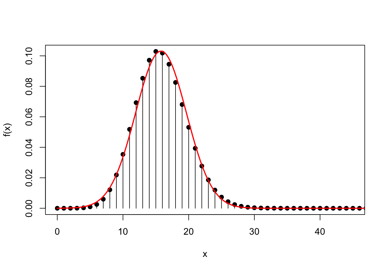
We approximate it by a normal distribution, choosing $\mu$ and $\sigma$ to match the expected value and standard deviation: \[\begin{align*} E[S] &= np = 300 \cdot \frac{2}{38} \approx 15.79 & \text{SD}[S] &= \sqrt{np(1-p)} = \sqrt{300 \cdot \frac{2}{38} \cdot (1 - \frac{2}{38})} \approx 3.87. \end{align*}\] So $S \approx \text{Normal}(\mu=15.79, \sigma=3.87)$. Now we can calculate $P(S \geq 22)$ using a normal distribution calculator:

# Python code
1 - Normal(mean=300 * 2/38, sd=sqrt(300 * 2/38 * (1 - 2/38))).cdf(22)

## 0.054161500900249515

# R
1 - pnorm(22, mean=300 * 2/38, sd=sqrt(300 * 2/38 * (1 - 2/38)))

## [1] 0.0541615

Notice that we plugged in 22 into the c.d.f. because the normal distribution is continuous. That is, \[ P(S \geq 22) = 1 - P(S < 22) = 1 - P(S \leq 22), \] since the probability that $S$ equals 22 exactly is zero. However, because we are using the normal distribution to approximate a discrete distribution, some people argue that we should plug in 21 or 21.5 instead. This is called a continuity correction, since it attempts to correct for the error in approximating a discrete distribution by a continuous one. Indeed, if you plug in 21.5, you get an approximation that is closer to the exact answer we obtained above.

# R
1 - pnorm(21.5, mean=300 * 2/38, sd=sqrt(300 * 2/38 * (1 - 2/38)))

## [1] 0.06990513

In my opinion, worrying about continuity corrections is like rearranging the deck chairs on the Titanic. There is no point in trying to make the normal approximation slightly better when you can just use a binomial calculator and get the exact answer. The normal approximation to the binomial is primarily interesting as an application of the Central Limit Theorem, not as a practical way to calculate probabilities.

Shown below is the normal approximation (in red) to the binomial p.m.f. (in black). The normal approximation is very good, but not perfect.

Essential Practice

There are 40 students in an elementary statistics class. From years of experience, the instructor knows that the time needed to grade a randomly chosen paper from an exam is a random variable with an expected value of 6 min and a standard deviation of 6 min.

If grading times are independent and the instructor begins grading at 8:00 p.m. and grades continuously, what is the (approximate) probability that she is done grading before the late night shows begin at 11:30 p.m.?
In roulette, a bet on a single number has a $1/38$ probability of success and pays 35-to-1. Consider betting on a single number on each of $n$ spins of a roulette wheel. Let $\bar X_n$ be your average net winnings per bet.
1. For which of the following values of $n$ is $\bar X_n$ close to normally distributed? Do a simulation to find out. (Copy the code below into a Colab and modify.)
```
# Python code (Make sure Symbulate has been imported.) 
n = 10
P = BoxModel({35: 1, -1: 37}, size=n, replace=True)
X = RV(P, mean)
X.sim(9999)
# You can use .plot() to make a histogram of these results.
```
```
# R code
n <- 10
replicate(9999,
          mean(sample(c(35, rep(-1, 37)), size=n, replace=TRUE)))
# You can use hist() to make a histogram of these results.
```
  - $n=10$
  - $n=100$
  - $n=1000$
  - $n=10000$
2. For each $n$, calculate the approximate probability that you come out ahead, i.e., $P(\bar X_n > 0)$. I encourage you to use a combination of simulation and the Central Limit Theorem (but first double check that it works!).
  
  (Hint: We calculated the expected value and variance of this bet in previous lessons.)
3. The casino wants to determine how many bets on a single number are needed before they have (at least) a 99% probability of making a profit. (Remember, the casino profits if you lose: $\bar X_n < 0$.) Determine the minimum number of bets, keeping in mind that $n$ must be an integer.
In San Luis Obispo, radioactive particles reach a Geiger counter according to a Poisson process at a rate of $\lambda = 0.8$ particles per second. What is the probability that the 100th particle is detected between 90 and 120 seconds? Calculate this probability in two ways:
1. Argue that the time the 100th particle is detected approximately follows a normal distribution. Use the normal approximation to calculate an approximate probability.
2. We derived the exact p.d.f. of the $r$th arrival time in Example 45.2. Integrate this p.d.f. to get the exact probability.
3. How good was the normal approximation?

Additional Practice

A randomly selected apple from the Cal Poly Orchard weighs 4.9 oz. on average, with a standard deviation of 0.3 oz. However, the distribution of the weights of apples is unknown.
1. With the information given, is it possible to determine the probability that a randomly selected apple weighs more than 5.0 oz? If so, calculate it.
2. The apples are packed into crates of 60 apples each. The apples are randomly and independently selected from the Cal Poly Orchard. With the information given, is it possible to determine the probability that the total weight of the apples in a crate exceeds 300 oz? If so, calculate it.